
A turbomolecular pump is a type of mechanical vacuum pump that is capable of reaching ultrahigh vacuum (UHV) conditions. Specialized numerical methods are required to model gas flows at such low pressures because the gas molecules rarely collide with each other. The COMSOL Multiphysics® software offers two distinct computational methods for the simulation of highly rarefied gases: the angular coefficient method and the Monte Carlo method. In this blog post, we introduce a Monte Carlo simulation of a turbomolecular pump stage.
Editor’s note: This blog post was originally published on August 9, 2017. It has since been updated to reflect new features and functionality.
Understanding Vacuum Systems
Vacuum technology is found in many high-tech industrial applications, such as the fabrication of semiconductor chips. Vacuum environments are also essential in fundamental research; for example, a particle accelerator would not work at atmospheric pressure because the particles being accelerated would collide with the surrounding air molecules much too often.
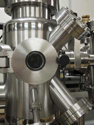
A typical vacuum chamber.
In a vacuum environment, the absolute pressure of the gas is much lower than the typical atmospheric pressure at sea level, which is about 101,325 pascals (Pa) or 14.7 pounds per square inch (psi). The atmosphere is mostly nitrogen and oxygen, but when dealing with vacuum chambers, we must consider every species involved. Even the outgassing (sublimation and evaporation) from walls, fittings, and lubricants can have a significant effect on the vacuum chamber pressure.
A vacuum pump is used to remove gas from the chamber, thereby reducing the chamber pressure. Many different types of vacuum pump are available, including:
- Rotary vane pumps
- Rotary piston pumps
- Diffusion pumps
- Turbomolecular pumps
- Cryogenic pumps
- Ion pumps
It is very common for two or more different varieties of pump to be used in tandem, each suited to a particular pressure range. For example, a rotary vane or piston pump can vent air at atmospheric pressure while reducing the vacuum chamber pressure to less than 0.1 Pa or so. A turbomolecular pump, on the other hand, can achieve UHV conditions (less than 10-7 Pa) but does not work properly at atmospheric pressure. To reduce the pressure all the way from atmospheric pressure to UHV, then, you could first reduce the pressure to 0.1 Pa using the rotary vane pump (called a roughing pump when used in this way) and then reduce the pressure from 0.1 Pa to 10-7 Pa using the turbomolecular pump.
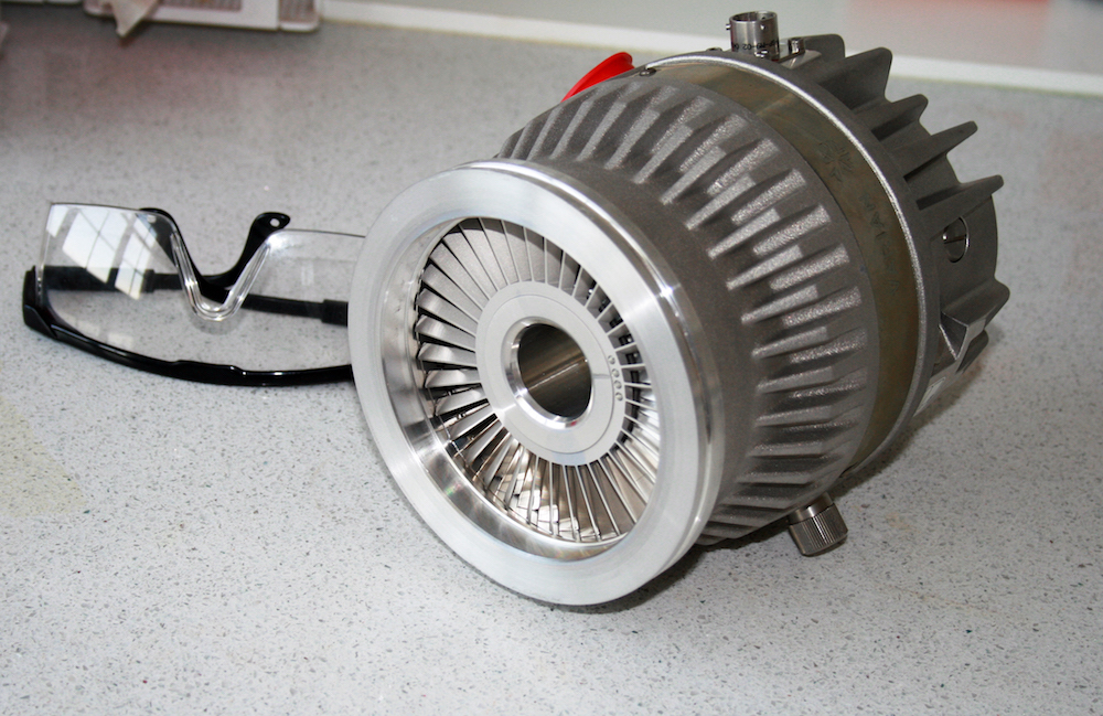
A turbomolecular pump.
Note that a perfect vacuum cannot be achieved in practice. A cubic meter of air at atmospheric pressure and room temperature has more than 10 septillion (1025) molecules. Even at UHV, a cubic meter of air still contains trillions of molecules! The goal is not to remove all of the air molecules, but just to remove enough of them so that they don’t impede the experiment or manufacturing process taking place inside the chamber.
Rarefied Gas Flows in Vacuum Systems
A turbomolecular pump will only work if the gas flowing through it is a free molecular flow. In other words, the gas pressure must already be low enough so that the molecules hit the surrounding surfaces much more frequently than they collide with each other. Therefore, this pump is only used to achieve UHV conditions after a roughing pump has already reduced the pressure to about 0.1 Pa.
Generally, when we think about airflow, we envision a continuum flow. When air flows into a room through a narrow passage, this puff of air spreads out and may create recirculation regions on all sides. When a stream of moving air reaches an obstruction, we expect it to flow around the obstruction, filling the empty space behind it. The air behaves in this way because the nitrogen, oxygen, and other gas molecules in air collide with each other billions of times per second.
At extremely low gas pressures, the gas behaves as a free molecular flow that is dominated by molecule-wall collisions instead of molecule-molecule collisions. If the gas is released into a large open space from a narrow aperture, then rather than spreading out in all directions due to intermolecular collisions, most of the molecules will fly out in nearly the same direction — a phenomenon called molecular beaming.
When the gas molecules strike a surface, they may get adsorbed by the surface or reflected away from it. Molecules are reflected by the surface in random directions even though the surface may appear perfectly smooth to the naked eye. A fair approximation is to assign a probability distribution to all of the different possible reflection angles. Usually, this probability distribution function is symmetric around the direction normal to the surface.
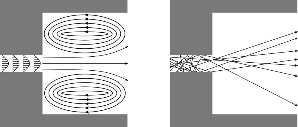
Comparison of a continuum flow (left) and a molecular flow (right) entering a chamber through a narrow tube.
Taking a Look Inside Turbomolecular Pumps
If you strike a ball with a flat board or a paddle, the ball will bounce in different directions depending on the angle of the paddle as it makes contact. This is the basic operating principle of a turbomolecular pump.
The pump consists of many rings, stacked on top of each other, all lined up along a common axis. Some of these rings rotate around the axis and are called rotors; others are held in a fixed position and are called stators. A typical design may contain many pairs of alternating rotors and stators. Within each ring are many narrow, inclined blades. Generally, each blade in the ring is inclined at the same angle and equally spaced, so if there are N blades, the ring has N-fold axial symmetry.
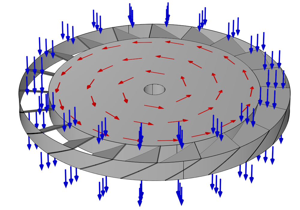
Because of the inclination of the blades in a rotor, when a molecule hits a blade, it is more likely to bounce out of the rotor in one direction than in the opposite direction. This behavior is illustrated in the following figure for a single rotor with no adjacent stators. Suppose this ring of blades is rotating counterclockwise, as indicated by the red arrows. It is more likely that a molecule will hit the underside of one of these blades rather than the top side. These molecules are then more likely to be deflected downward (in the direction of the blue arrows) than in the opposite direction. Because of this preferential deflection of molecules in a downward direction, the air pressure in the region above this rotor can be reduced.
For the difference in transmission probability (top to bottom versus bottom to top) to be significant, the blade surfaces should move at a speed comparable to or greater than the mean thermal velocity of the molecules. This speed is on the order of several hundred meters per second for most gases at room temperature, but is significantly greater for very light gases such as hydrogen. Thus, when using a turbomolecular pump to reduce the chamber pressure down to UHV, most of the residual gas in the chamber will be hydrogen (Ref. 1).
The blades of a turbomolecular pump are organized into units called stages. A typical pump stage might contain 8–20 rings of such blades (Ref. 2), alternating between rotors and stators. For simplicity, our current model only considers a single rotor.
When setting up a numerical model of a turbomolecular pump, the main purpose is usually to predict its pumping speed and pressure ratio. These can be predicted from the transmission probability of molecules across the ring of blades — that is, the fraction of molecules that exit through the bottom after entering the stage from the top, and vice versa.
Choosing a Numerical Method
In the COMSOL® software, there are two main numerical methods for simulating extremely rarefied gas flows. One is called the angular coefficient method and is used by the Free Molecular Flow physics interface, available with the Molecular Flow Module. The angular coefficient method is a sort of view factor calculation that computes molecular fluxes at boundaries in the model, assuming that the gas molecules will only collide with walls and never with other molecules. The main drawback of the angular coefficient method is that it is “quasistationary” — that is, it ignores the finite time-of-flight of the molecules, which is an important factor here because the blades can easily reach speeds of several hundred meters per second, comparable to the molecular speeds.
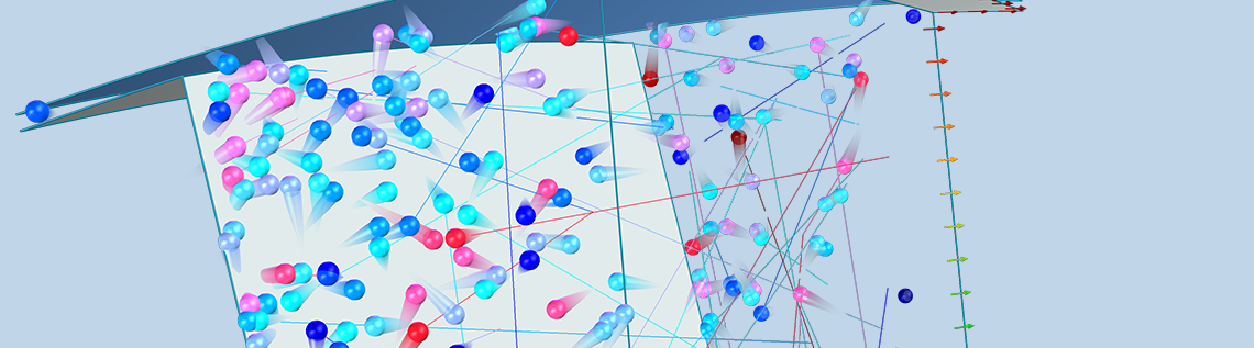
In order to fully account for the motion of the blades in the turbomolecular pump, we will instead be performing a Monte Carlo simulation using the Mathematical Particle Tracing interface available with the Particle Tracing Module. In a Monte Carlo model, we solve for the motion of individual molecules in the gas by solving Newton’s laws of motion. The true number of individual molecules in the pump might be far too large to model each molecule individually, due to limitations in computational cost, but we can take a representative sample of the molecules — say 100,000 — and then extrapolate the results for the entire population of molecules.
A Monte Carlo simulation is used to predict the transmission probability of gas molecules across a simplified turbomolecular pump stage, consisting of a single rotating ring of blades. As we discussed earlier, a typical pump rotor containing N blades will usually exhibit N-fold rotational symmetry. Therefore, we can further simplify the model and reduce the computational cost by only considering the molecules that pass through a single gap between two adjacent blades.
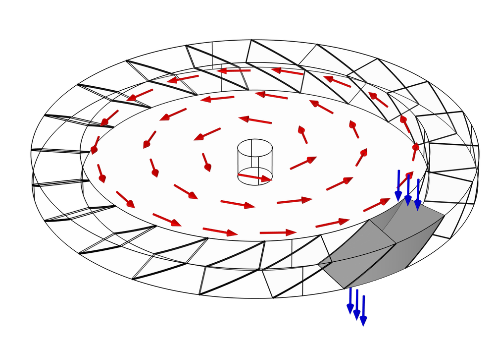
The gap between the blades is also bounded by two cylindrical surfaces, the inner root wall and the outer tip wall. You might notice from the previous two figures that the actual space that the molecules can travel through is not the full disk, but just an annular region some distance away from the axis of rotation. This is because the velocity of any point on the blade is proportional to its radial distance from the center,
So, no matter how fast the rotor spins, you’d get diminishing returns from trying to move the root wall closer to the axis of rotation.
The practical limit on the angular velocity is somewhat less than 100,000 revolutions per minute (Ref. 1).
Choosing a Frame of Reference
At this point, our simulation domain is just the empty space bounded at the front and the back by the adjacent blades, and on the left and right by the root and tip walls. Gas molecules may enter the domain from both the top and bottom, and our objective is to determine what fraction of molecules released from the top will exit out the bottom, and vice versa.
Here, we encounter another technical challenge: The space between the rotor blades is moving around in a circle. When modeling in a moving domain, you must decide what frame of reference to use in the model. Usually, the choice is one of the following:
- Set up the model in the “laboratory” frame of reference. That is, model the rotor from the point of view of an observer standing motionless outside of it and watching it spin. To do so, you’d have to explicitly cause the geometry to rotate over time, perhaps using the dedicated Rotating Domain node. From this point of view, molecules follow straight-line paths as they move from one surface to the next.
- Set up the model in a moving frame of reference attached to the rotor. That is, imagine how the molecule trajectories would look if we, the observers, could shrink down and ride one of these rotor blades. In this frame of reference, the paths followed by individual gas molecules may appear to be curved.
In this example, we’ll be using the second approach. However, this brings up an additional complication, as we’ll see below.
Particle Tracing in a Rotating Frame of Reference
The molecules obey Newton’s second law of motion,
where q is the particle position, mp is the particle mass, and Ft is the sum of all applied forces.
In this example, we neglect gravity, so the net force is zero. But Newton’s second law of motion is formulated in an inertial frame of reference, meaning that it will hold true only if the observer is not accelerating. Rotation is a kind of acceleration, so this model is set up in a noninertial frame of reference.
As another way of visualizing inertial vs. noninertial frames, imagine trying to perform a simple physics experiment (say, bouncing a ball or tracking the motion of a pendulum) while on the back of a moving truck. Such an experiment would give the same result if the truck were parked or if it were being driven in a straight line with the cruise control on. But, the experiment would give different results if the truck were speeding up, slowing down, or turning.
If the distance from the root wall to the tip wall is much smaller than the distance from the axis of rotation to the root wall — that is,
then we may, as a first approximation, just ignore the fact that our frame of reference is noninertial.
This is equivalent to treating the ring of blades as if it were actually an infinite straight line of blades, all moving in the same direction. This assumption is made in the Quasi-2D Turbomolecular Pump tutorial model and discussed further in Ref. 3. This simplifying assumption greatly reduces the computational effort involved because it causes the particles to move in straight lines in the frame of reference attached to the blades. This is a fair approximation when the rotor is turning slowly, but it becomes less accurate as the angular velocity of the rotor is increased.
To perform a high-fidelity Monte Carlo simulation, we must respect the fact that our frame of reference is rotating. Fortunately, the Mathematical Particle Tracing interface already provides a dedicated physics feature specifically for this purpose. You can add the Rotating Domain node to your model to define the fictitious forces that arise from tracing particles in a rotating frame of reference,
\mathbf{F}_\textrm{t} &= \mathbf{F}_\textrm{cen} + \mathbf{F}_\textrm{cor}\\
\mathbf{F}_\textrm{cen} &= m_\textrm{p}\mathbf{\Omega}\times\left(\mathbf{q}\times\mathbf{\Omega}\right)\\
\mathbf{F}_\textrm{cor} &= 2m_\textrm{p}\mathbf{v}\times\Omega
\end{align}
These fictitious forces are called the centrifugal force Fcen and the Coriolis force Fcor. In these equations, v is the particle velocity and Ω is the angular velocity of the rotating frame. For simplicity, it is assumed here that the axis of rotation passes through the origin.

Settings for the Rotating Frame node.
Particle Release and Boundary Conditions
By adding the Rotating Domain node to the model, both the centrifugal and Coriolis forces will be automatically defined. All that remains is to define the particle release and boundary conditions.
The molecules are released into the simulation domain using Inlet nodes on the top and bottom boundaries. This model uses the Thermal velocity distribution, in which the initial speed of each molecule is sampled from a Maxwell distribution and its initial direction is sampled following the cosine law.
The blade velocity is then subtracted from the velocity of the released molecules because the gas in the region adjacent to the pump stage has zero drift velocity in the laboratory frame of reference.

Settings for the Inlet node.
The blade walls, root wall, and tip wall all use the Thermal Reemission boundary condition. Whenever a molecule hits one of these surfaces, it bounces back into the domain with a new random speed and random direction. The blade walls and root wall are assumed to move with the rotating frame, while the tip wall is assumed to be fixed in the laboratory (inertial) frame. A built-in setting is used to subtract the moving frame velocity from the reinitialized particle velocity for any molecules that hit the tip wall.

Settings for the Thermal Reemission node at the tip wall.
Results
The transmission probability is defined as the fraction of the released molecules that will cross from one side of the pump stage to the other, rather than being knocked backward by the blades. When the blades are rotating, we can define two distinct transmission probabilities: the transmission probability in the forward direction (top to bottom in the previous diagrams) and in the reverse direction (bottom to top).
From the transmission probability of the molecules in the forward and reverse directions, we obtain the maximum compression ratio Kmax and the maximum speed factor Wmax,
where M12 is the transmission probability in the forward direction and M21 is the transmission probability in the reverse direction.
Let’s look at some plots comparing these transmission probabilities to a dimensionless velocity ratio C. This is the ratio of the blade speed (measured at the root mean square or rms radius) to the most probable speed of the molecules in the gas. The molecule speed is a function of molecule mass and gas temperature. In general, molecules move faster in a hotter gas, and lighter molecules move faster than heavier ones. For this reason, turbomolecular pumps are better at pumping out heavier species like argon, nitrogen, and oxygen, but they’re somewhat less efficient at pumping hydrogen (Ref. 2).
When the blades are at rest (C = 0), the transmission probabilities for the forward and reverse directions are roughly equal. As the blades begin to spin faster, the probability in the forward direction approaches unity while the probability in the reverse direction approaches zero.
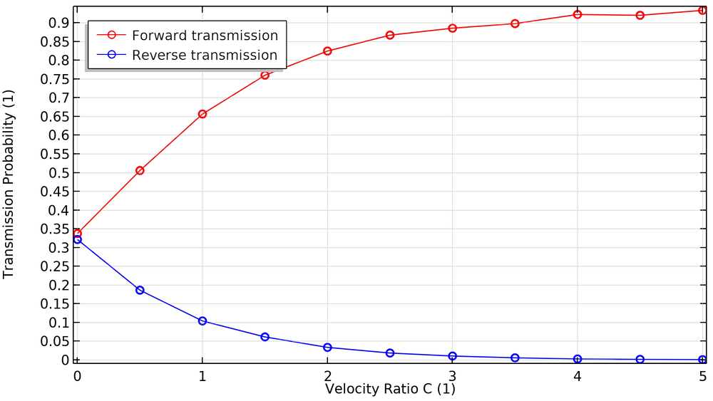
The fraction of particles transmitted in the forward and reverse directions as a function of blade velocity ratio.
We also investigate how the compression ratio and pumping speed are affected by the blade velocity ratio. To produce enough compression and speed, pumps use multiple bladed structures comprised of several disks and different types of blades. Blades close to the chamber inlet are designed to have a high pumping speed and low compression ratio, while blades close to the foreline (the connection to the roughing pump) are designed to have a low pumping speed and a high compression ratio.
When the velocity of these blades increases, as seen in the plots below, the maximum compression and speed factor increase. These plots show excellent agreement with a similar study reported in Ref. 4.
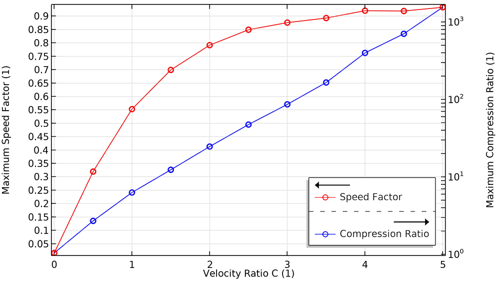
The effect of blade velocity on the maximum compression ratio and maximum speed factor.
Next Steps
This example highlights several features that make it easier to perform Monte Carlo simulation of turbomolecular pumps. Try it yourself by clicking on the button below.
Learn More About Particle Tracing in COMSOL Multiphysics®
Check out these blog posts on particle tracing:
- Benchmark Model Shows Reliable Results for Inertial Focusing Analysis
- Sampling Random Numbers from Probability Distribution Functions
References
- J.M. Lafferty, ed., Foundations of Vacuum Science and Technology, John Wiley & Sons, 1998.
- J.F. O’Hanlon, A User’s Guide to Vacuum Technology, 3rd ed., John Wiley & Sons, 2003.
- S. Katsimichas, A.J.H. Goddard, R. Lewington, and C.R.E. De Oliveira, “General geometry calculations of one-stage molecular flow transmission probabilities for turbomolecular pumps,” Journal of Vacuum Science & Technology A: Vacuum, Surfaces, and Films, vol. 13, no. 6, pp. 2954–2961, 1995.
- Y. Li, X. Chen, Y. Jia, M. Liu, and Z. Wang, “Numerical investigation of three turbomolecular pump models in the free molecular flow range,” Vacuum, vol. 101, pp. 337–344, 2014.

Comments (0)