
Inertial focusing is a useful technique for various applications, particularly within the medical field. Ensuring its effectiveness requires accurately describing the migration of particles as they flow through a channel. Version 5.3 of the COMSOL Multiphysics® software gives you the tools to generate reliable results that agree with experimental data on inertial focusing. Our new benchmark model highlights these capabilities.
The Power of Inertial Focusing
In the 1960s, G. Segré and A. Silberberg observed a surprising effect: When carried through a laminar pipe flow, neutrally buoyant particles congregate in a ring-like structure with a radius of about 0.6 times the pipe radius. This correlates to a distance from the parallel walls of around 0.2 times the width of the flow channel. The reason for this behavior, as they would discover decades later, could be traced back to the forces that act on particles in an inertial flow.
Today, we use the term inertial focusing to describe the migration of particles to a position of equilibrium. This technique is widely used in clinical and point-of-care diagnostics as a way to concentrate and isolate particles of different sizes for further analysis and testing.

Many types of medical diagnostics use inertial focusing for testing and analysis. Image in the public domain, via Wikimedia Commons.
In order for inertial focusing to be effective in these and other applications, accurately analyzing the migration patterns of the particles is a key step. A new benchmark example from the latest version of COMSOL Multiphysics — version 5.3 — highlights why the COMSOL® software is the right tool for obtaining reliable results.
Accurately Model the Migration of Particles in Inertial Focusing
For this example, we consider the particle trajectories in a 2D Poiseuille flow. To account for relevant forces, we use derived expressions from a similar migration of particles in a 2D parabolic flow inside of two parallel walls (see Ref. 2 in the model documentation). Built-in corrections for both the lift and drag forces allow us to account for the presence of these walls in the simulation analysis.
Note: Lift and drag forces make up the total force acting on neutrally buoyant particles inside a creeping flow. By definition, the gravitational and buoyant forces cancel out one another.
We assume that the lift force acts only perpendicular to the direction of the fluid velocity. It is also assumed that the spherical particles are small in comparison to the width of the channel and that they are rotationally rigid.
To compute the velocity field, we use the Laminar Flow physics interface. This is then coupled to the Particle Tracing for Fluid Flow interface via the Drag Force node. Thanks to the Laminar Inflow boundary condition, we can automatically compute the complete velocity profile at the inlet boundary. For the laminar flow of a Newtonian fluid inside two parallel walls, it is known that the profile will be parabolic. This means that we could have directly entered the analytic expressions for fluid velocity. However, we opt to use the Laminar Flow physics interface in this case, as it demonstrates the workflow that is most appropriate for a general geometry.
Now let’s move on to the results. First, we can look at the fluid velocity magnitude in the channel. As expected, the velocity profile is parabolic. Note that the aspect ratio of the geometry is 1000:1, so the channel is very long compared to its height. The plot uses an automatic view scale to make the results easier to visualize.
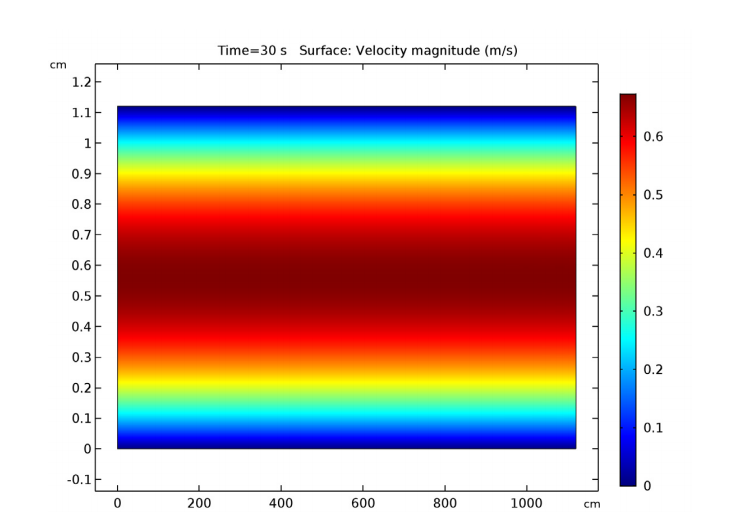
The parabolic fluid velocity profile within a channel that is bound by two parallel walls.
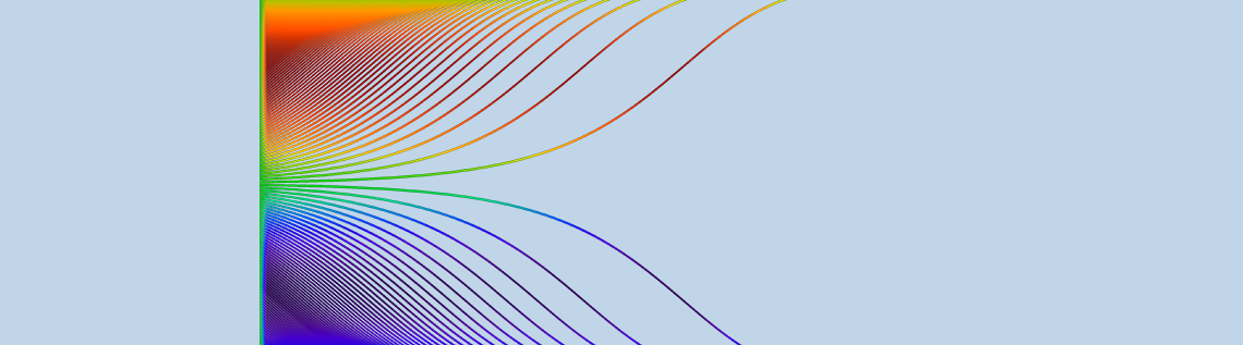
We can then shift our attention to the trajectories of the neutrally buoyant particles. Note that in the plot below, the color expression represents the y-component of the particle velocity in mm/s. The results indicate that all of the particles are close to equilibrium positions at distances of about 0.3 D on either side of the center of the channel. (D represents the width of the channel). It does, however, take longer for particles released near the center of the channel to reach these positions. Their initial force is weaker as they are released in the area where the velocity gradient is smallest. From the plots, we can see that the particles converge at heights that are 0.2 and 0.8 times the width of the channel. These findings show good agreement with experimental observations.
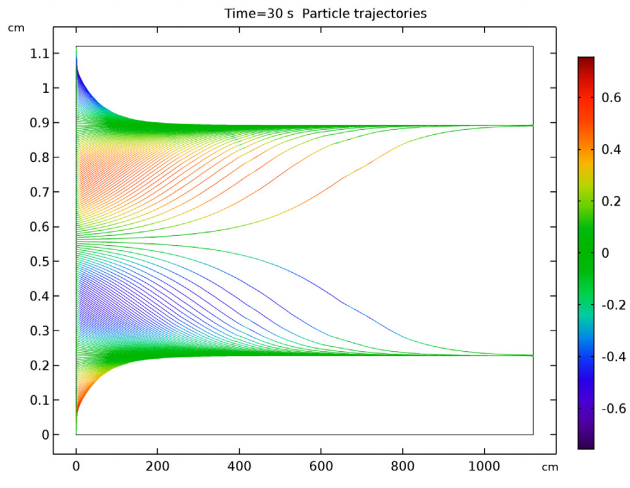
The trajectory of particles inside the channel.
The last two plots show the average and standard deviation of the normalized distance between the particles and the center of the channel. These results verify that the equilibrium distance from the center of the channel is in fact around 0.3 D.


The average (left) and standard deviation (right) of the normalized distance between the particles and center of the channel.
Generating Reliable Results for Inertial Focusing Studies
In order to effectively use inertial focusing for medical and other applications, you need to first understand the behavior of particles as they migrate through a channel to positions of equilibrium. With COMSOL Multiphysics® version 5.3, you can perform these studies and generate reliable results. This accurate description of inertial focusing serves as a foundation for analyzing and optimizing designs that rely on this technique.
Now it’s your turn! Give our new benchmark model a try:
Interested in learning about further updates in version 5.3 of COMSOL Multiphysics? You can get the full scoop in our 5.3 Release Highlights.


Comments (6)
Ivana Milanovic
May 29, 2017Hi Bridget,
How did you accomplish rainbow coloring for particles? I see just individual colors in C5.3.
Thanks,
Bridget Cunningham
June 6, 2017Hi Ivana,
Thanks for your comment.
To color particles according to arbitrary expression (the y-component of the velocity in the above example), simply right click on the Particle Trajectories 1 plot and select “Color Expression”. The color scheme in the blog post can be selected by setting the “Color table” to “Spectrum”.
You could also open the example model via File > Application Libraries > Particle Tracing Module > Fluid Flow > inertial focusing.
Mehran Hoonejani
July 24, 2017Hi Bridget,
Can this wall-induced lift force be used in 3D too? What surfaces should be selected as parallel walls for, say, duct flow or flow in a cylinder?
Thanks
Bridget Cunningham
July 25, 2017Hi Mehran,
Thank you for your comment.
It should work in duct flows between parallel walls, but not for flow in cylindrical pipes.
If you have additional questions related to your modeling, please contact our Support team.
Online Support Center: https://www.comsol.com/support
Email: support@comsol.com.
Songtao Ye
February 10, 2020I know we have wall-induced lift force and staffman lift force. But how do we include the shear-gradient induced lift force (i.e. to get the net inertial lifting force) in the particle tracing model?
Brianne Christopher
February 10, 2020Hello Songtao,
Thank you for your comment.
For questions related to your modeling, please contact our Support team.
Online Support Center: https://www.comsol.com/support
Email: support@comsol.com