

Here is an interesting question: How can we easily probe the solution at a point that is moving in time, but associated with a stationary geometry? One option is to use the General Extrusion coupling operator. In this blog post, we will take a look at how to use the General Extrusion coupling operator to probe a solution at a point in your geometry, and illustrate how to implement a dynamic probe using an example model.
Computing the Laser Heating of a Rotating Silicon Wafer
Let’s consider a laser heating example where you have a moving heat source, the laser, and a moving geometry. The model in question is called Laser Heating of a Silicon Wafer, and can be found in the Model Gallery. In this model, a laser moves radially inwards and outwards over a silicon wafer that is rotating on its stage. The incident heat flux from the laser is modeled as spatially varying, with time varying coordinates for the location of the incident heat flux. The effect of the rotation of the wafer is modeled through a transport term in the governing heat transfer equation:
The transport term in this equation, \bf{u}, is used to account for the rotation of the wafer, so it is not necessary to explicitly rotate the geometry.
Now suppose we would like to evaluate the temperature at one point of the rotating wafer. We are then looking at the problem of evaluating the temperature at a point that follows the rotating wafer material. This problem can be solved by using a General Extrusion coupling operator to dynamically map the solution at a particular point (moving or stationary) onto a fixed source.
We begin by adding the General Extrusion coupling operator from the definitions toolbar as shown in the screenshot below:
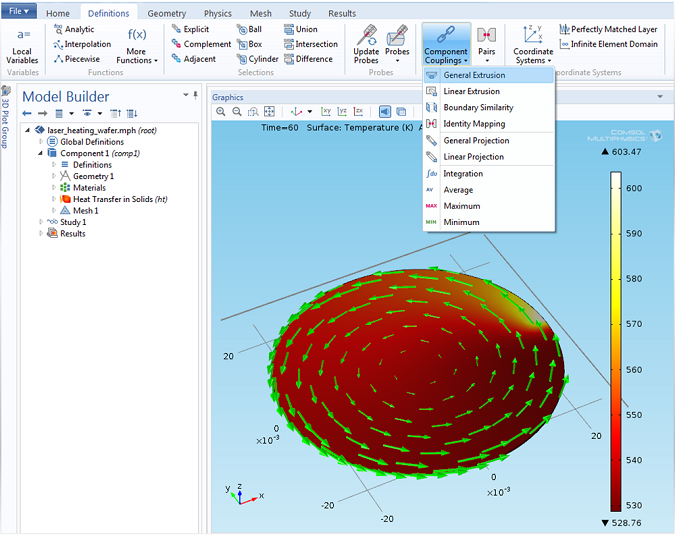
Adding a General Extrusion coupling operator.The green vector field is the transport term used to model the wafer rotation.
Next, let’s take a look at the settings of the General Extrusion coupling operator. The time varying coordinates of the point at which we want to evaluate the temperature can be entered as the coordinates of the destination map. Let’s consider a point on the disk at a distance of 0.5 inches from the center of the disk located at (0,0). At any given time, the (x, y, z) coordinates of this point are given by: (0.5[in]*cos(ωt), 0.5[in]*sin(ωt), 2.75e-4[m]), where ω is the angular velocity of the rotating wafer disk. We can simply enter the time varying coordinates in the x, y, and z-expressions of the destination map. In general, the destination map accepts scalar values that may be space- or time-dependent expressions. The settings of the General Extrusion coupling operator are shown below:
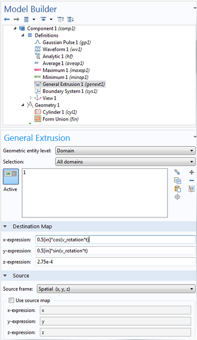
General Extrusion coupling operator settings. A destination map and source map is specified here. The destination map here consists of the transient coordinates where we would like to evaluate temperature.
Note that the operator name is kept to its default: genext1. In this example, since the x, y, and z-coordinates of the destination map are explicitly specified without any association with the coordinates of a geometric entity, it doesn’t matter where we evaluate the General Extrusion coupling operator. It will always be requested to be evaluated at the destination coordinates entered in the settings of the General Extrusion coupling operator. To evaluate the temperature at the destination coordinates, you can call the General Extrusion coupling operator with a temperature argument, as genext1(T), where T is the dependent variable name for Temperature. If you have already computed the solution to the finite element problem, then you can simply evaluate temperature at the destination points by clicking on the “update solution” option in the Study toolbar, or you can dynamically probe the variable genext1(T) evaluated at a point while you compute the solution to the finite element problem.
The plot below shows the graph for temperature evaluated at a point located 0.5 inches from the center of the rotating disk:
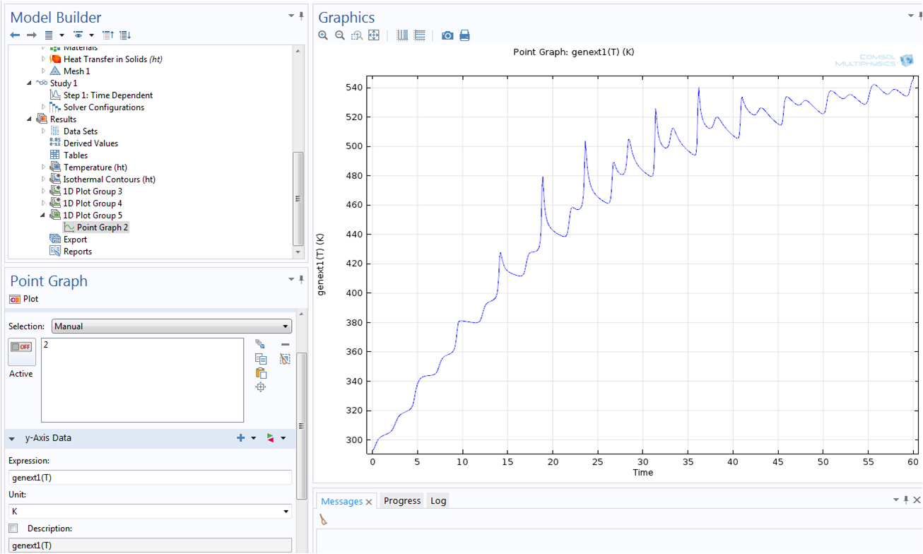
Temperature evaluated at a point on the rotating wafer.
We can similarly evaluate the temperature at any other point. All you need are the time-dependent coordinates of the point where you would like to evaluate the temperature. For example, if you would rather follow the point on the geometry that corresponds to the focal point of the moving laser, you would enter the time-varying coordinates of the focal point of the laser.
The plot below shows the temperature evaluated at the focal point of the moving laser:
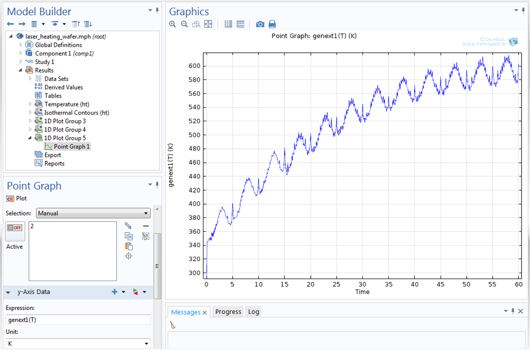
Temperature evaluated at a point on the geometry corresponding to the focal point of the moving laser.
Next Steps: Mapping Cross-Sectional Data
Now you know how to use the General Extrusion coupling operator to probe a solution at a moving point. In an upcoming blog post, we will walk you through how to use the operator to map cross-sectional data from one or several cross sections onto another cross section for geometries where the cross section dimensions do not change over the length of interest. This will allow you to compare different cross-sectional data and evaluate measures such as maximum, minimum, and average over several cross sections. Stay tuned!

Comments (7)
Dong Liu
June 10, 2014I am also troubled by such a problem of time-dependent coordinates. I tried to use your method but I failed. have some questions. How did you select the source in the general extrusion settings? Why are all the domains selected? In the results, how is Point 2 related to the general extrusion?
Chandan Kumar
June 12, 2014Dear Dong,
The source domain(s) can be the domain(s) on which the destination point(s) are defined. I suppose by “point 2” you are referring to the second plot. point 2 there simply involves time varying coordinates of the focal point of the laser beam in the example model : http://www.comsol.com/model/laser-heating-of-a-silicon-wafer-13835
Best regards,
Chandan
Charles Selfridges
July 23, 2014Dear Chandan,
I wonder when will you post about “Mapping Cross-Sectional Data”? I hope I have not missed it.
Best regards,
Charles
Raghavendran Raman
March 6, 2019Hi,
I am trying to use the same for droplet evaporation. I need to obtain a whole bunch of data in the variables section, ef., Mass fraction, Density and others. I defined a general extrusion operator, then defined variables such as T_sf = genext1(comp1.T), Y_sf = genext1(Y) and so. unfortunately, I get the following error,
Unknown function or operator.
– Name: genext1
Can you help me out?
Thanks and regards,
Raghavendran Raman
Brianne Christopher
March 12, 2019Hello Raghavendran,
Thank you for your comment.
For questions related to your modeling, please contact our Support team.
Online Support Center: https://www.comsol.com/support
Email: support@comsol.com
博 张
August 11, 2019Hi, Raghavendran,
I guess your problem is that there is no recalculation after defining genext1, and this error will not be prompted after the calculation.
Hope can help you.
Bo Zhang
Mirza Sahaluddin
March 12, 2023This worked perfectly for a point moving on a surface. However, this approach did not work for a point moving on a surface that is between two domains, i.e. at an interface. I would appreciate any help. Thank you! Also, are there other approaches to do this?