Metal Processing Module
COMSOL Multiphysics® version 5.5 introduces the new Metal Processing Module. This add-on module allows you to model metallurgical phase transformations in materials like steel and cast iron.
Metal Processing Module Overview
The Metal Processing Module brings two new physics interfaces, Metal Phase Transformation and Austenite Decomposition for analyzing metallurgical phase transformations. Both of these interfaces provide functionality to model diffusive as well as displacive phase transformations. As with all COMSOL Multiphysics® add-on modules, the Metal Processing Module was developed with multiphysics in mind.
The module provides more sophisticated heat transfer functionality when combined with the Heat Transfer Module, with the ability to compute effective thermal material properties as well as phase transformation latent heat and the effects of heat radiation. Similarly, by combining it with the Structural Mechanics Module and its add-on modules, you can compute residual stresses, phase transformation strains, and deformations. The Metal Processing Module can also compute effective mechanical material properties and phenomena like transformation-induced plasticity (TRIP), and thermal strains can be included.
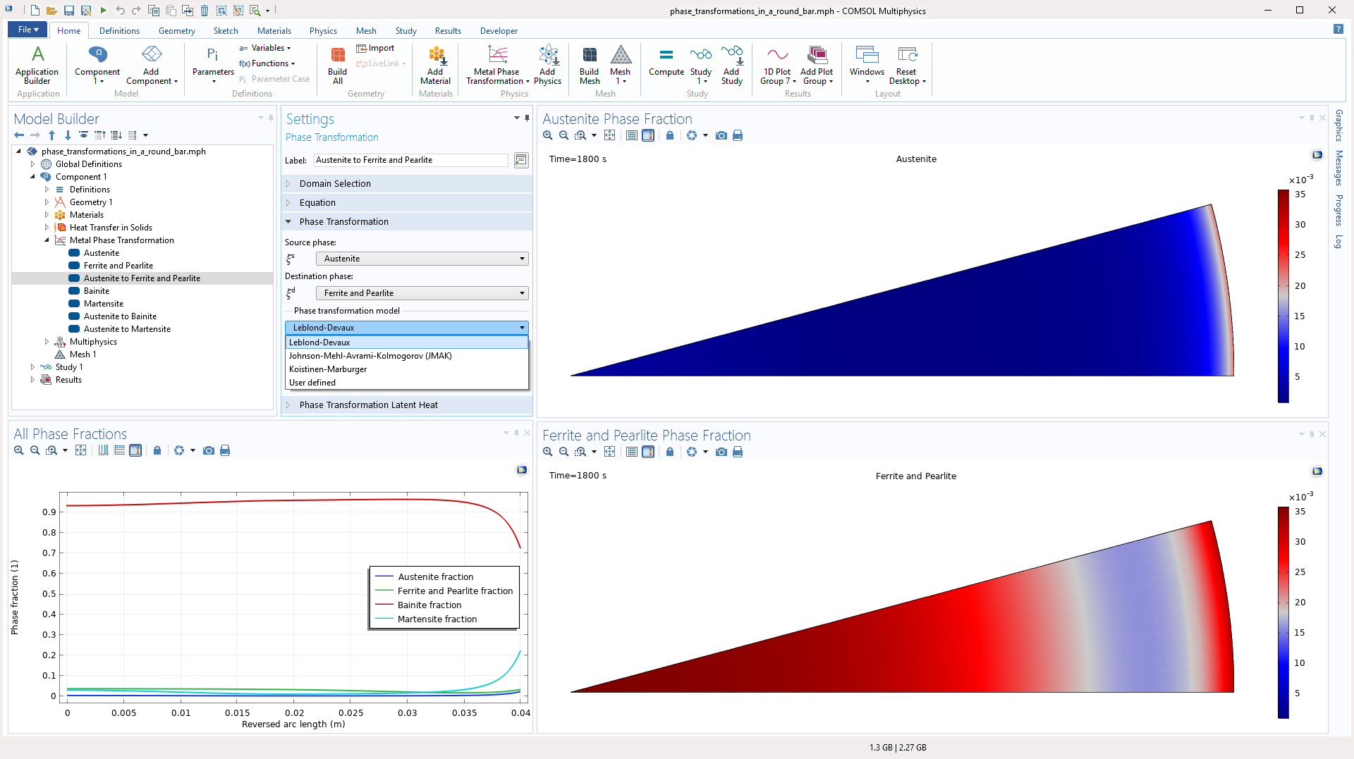
The Metal Phase Transformation Interface
The Metal Phase Transformation interface is used to study metallurgical phase transformations that occur in a material like steel, during heating or cooling, by computing the evolving phase composition in components like transmission gears, shafts, and axles during heat treatment. The Metallurgical phase feature is used to define the initial phase fraction and material properties, and the Phase transformation feature is used to define the source phase, destination phase, and phase transformation model. When the interface is added, two Metallurgical phase nodes and one Phase transformation node are automatically generated, as that is the minimum requirement to set up such a model. You can then define an arbitrary number of additional phases and phase transformations in your model.
Three types of phase transformation models are provided:
- The Leblond–Devaux model
- The Johnson–Mehl–Avrami–Kolmogorov (JMAK) model
- The Koistinen–Marburger model
The first two models are suitable for diffusion–controlled phase transformations, such as when austenite decomposes into ferrite. The last model is suitable to model the displacive (diffusionless) martensitic phase transformation. In addition to these models, you can define your own phase transformation models.
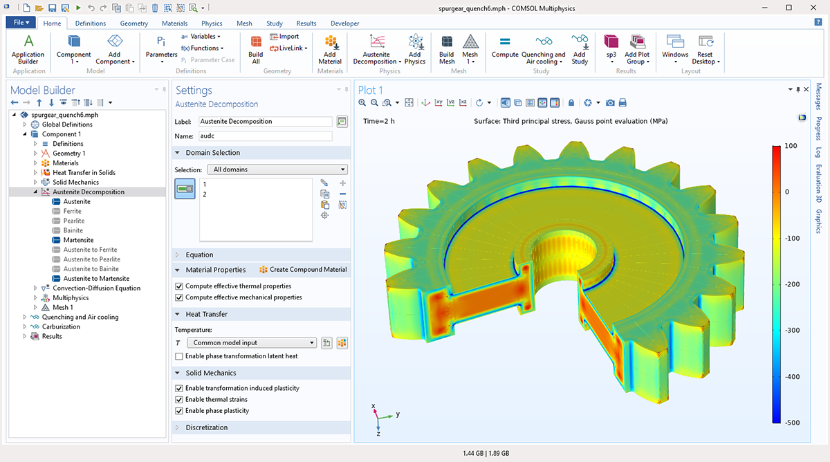
The Austenite Decomposition Interface
The Austenite Decomposition interface is based on the Metal Phase Transformation interface, but specialized to simulate the quenching of steels. As such, the Metallurgical Phase and Phase Transformation Model Builder tree nodes that represent the most common phase transformation processes during austenite decomposition are automatically generated when the interface is added. Using the Austenite Decomposition interface, you can compute how the phase composition evolves over time, at certain locations in a component, and compute the residual stress state after quenching.
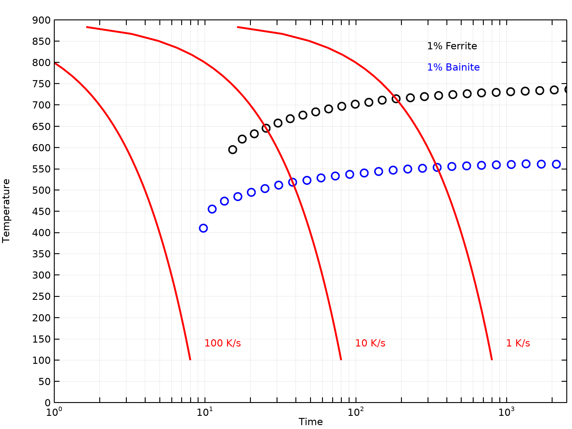
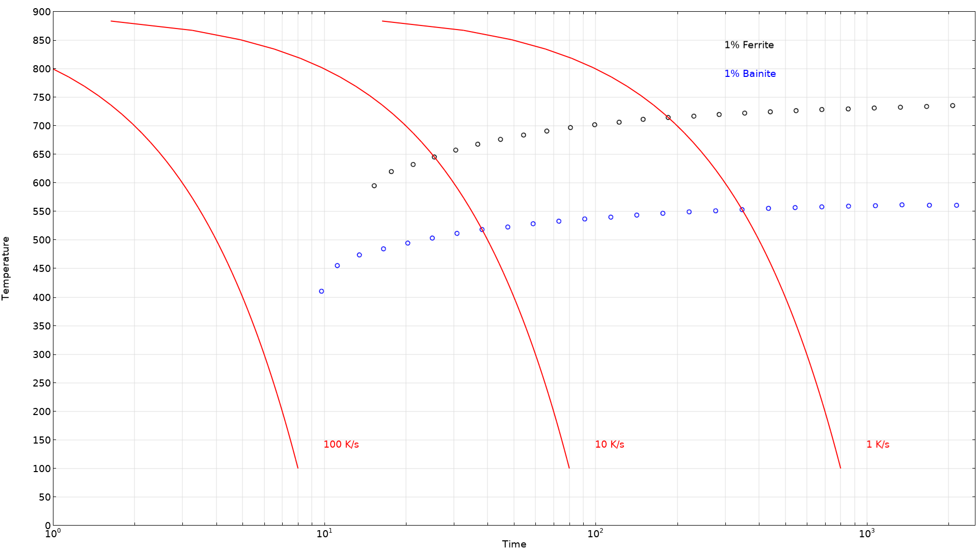
Calibration of Phase Transformation Models
Experimental calibration is required for a given phase transformation. Using the Metal Phase Transformation and Austenite Decompositon interfaces, you can compute common phase transformation diagrams to facilitate calibration against experimental data. A computed continuous cooling transformation (CCT) diagram is exemplified in the Transformation Diagram Computation model.
Multiphysics Functionality
The Metal Processing Module provides two multiphysics coupling nodes to facilitate coupling to the Heat Transfer in Solids and Solid Mechanics interfaces. The Phase Transformation Latent Heat multiphysics coupling is used to include heat released or absorbed during metallurgical phase transformations. The Phase Transformation Strain multiphysics coupling is used to include TRIP, plasticity of the individual metallurgical phases, and thermal strains. The multiphysics couplings can be used with both the Metal Phase Transformation and Austenite Decomposition interfaces. Additionally, the Metal Processing Module can be used together with the AC/DC Module to model induction hardening, and processes like carburization can be modeled as a general diffusion problem.
Example Tutorial Models
The Metal Processing Module includes four fully documented tutorial models to demonstrate the features and functionality available.
Transformation Diagram Computation
Application Library Title:
transformation_diagram_computation
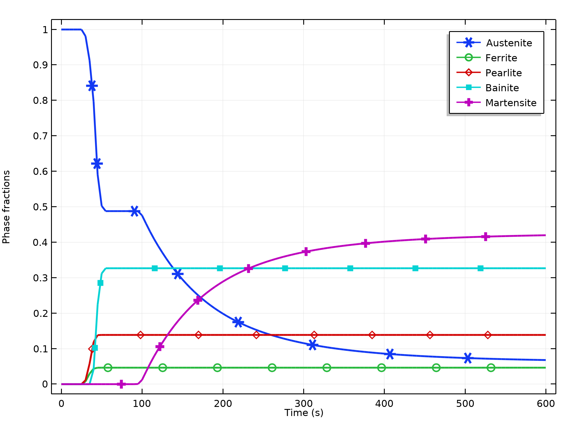
Phase Transformations in a Round Bar
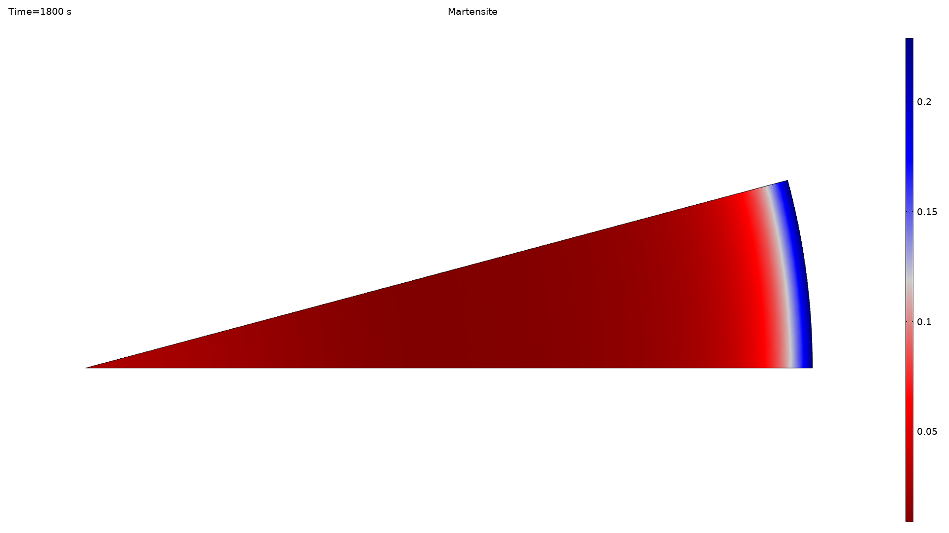
Application Library Title:
phase_transformations_in_a_round_bar
Quenching of a Steel Billet
Application Library Title:
quenching_of_a_steel_billet
Carburization and Quenching of a Steel Gear
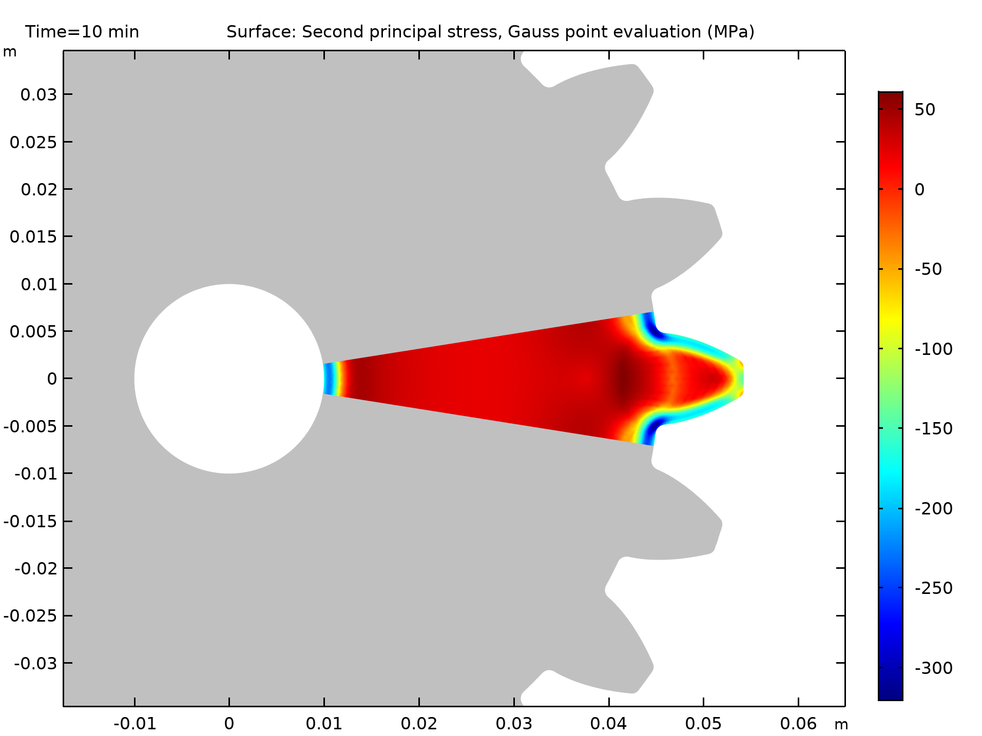
Application Library Title:
carburization_and_quenching_of_a_steel_gear