

Composites are widely used in industrial applications. Compared to the traditional monolithic materials, composites can have specialized material properties due to the customization of constituents, making them versatile and applicable to many different industries, such as in areas like aerospace engineering and biomedical engineering. Homogenization techniques are needed to numerically compute the material properties of composites and can be used for the customization and design of versatile materials. In this blog post, we are going to look at a simulation app developed in the COMSOL Multiphysics® software using the Application Builder that can be used for composite material design and material homogenization.
This blog post provides an introduction to the material homogenization app. If you want a more technical introduction to material homogenization in general, check out our Learning Center article “Homogenization of Material Properties”.
Introduction to Homogenization
Before we start discussing the homogenization app, let’s go over the important modeling steps for homogenization. The 4 key steps are:
- Creating the geometry of a repeating unit cell (RUC)
- Assign material properties to the constituents
- Apply periodic boundary conditions
- Retrieve the homogenized material properties
Now, we’ll take a closer look at each of these steps.
Step 1: Repeating Unit Cells
The first step is to generate a geometry of a RUC in the model builder in COMSOL Multiphysics®. You can import a geometry, build it, or use one of the RUC geometries available in the COMSOL Multiphysics Part Libraries.
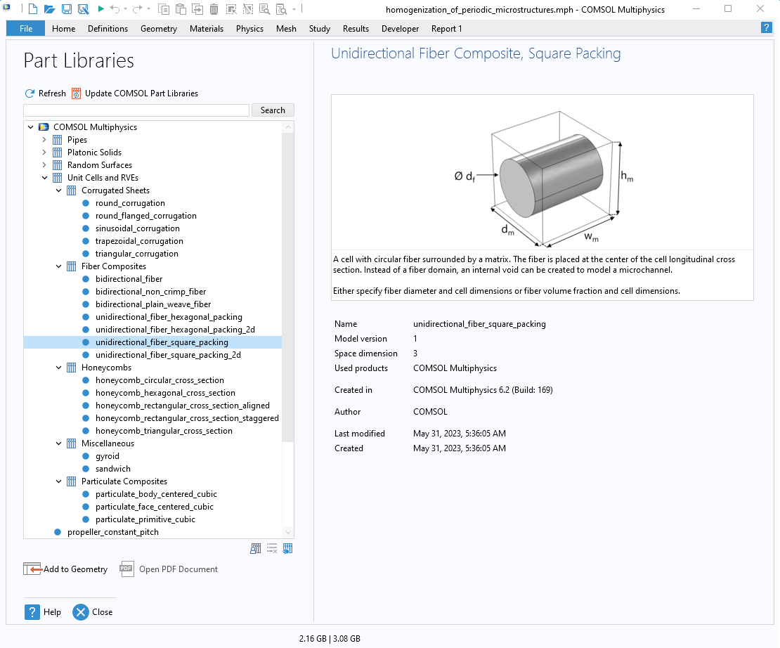
Example of a RUC geometry in the Part Libraries.
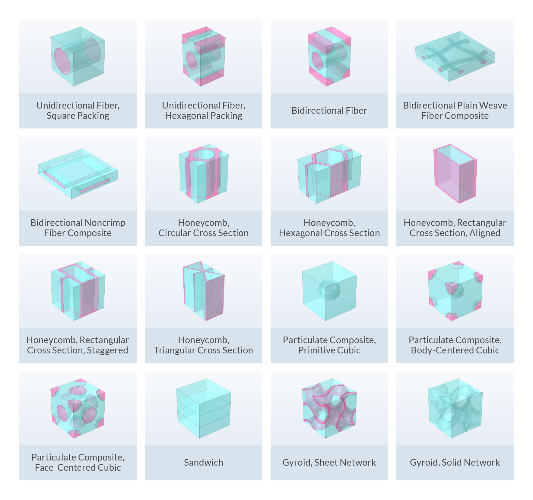
The available geometry parts for different RUCs are shown below.
Step 2: Constituents Material Properties
The constituent material properties can be assigned using the Materials node in the Model Builder in COMSOL Multiphysics®.
Step 3: Periodic Boundary Conditions
In the Solid Mechanics interface, the Cell Periodicity feature has built-in periodic boundary conditions for computing the homogenized elasticity tensor, compliance tensor, coefficient of thermal expansion, and coefficient of hygroscopic swelling. In the Boundary Conditions settings, there are three options for how the homogenized properties are computed:
- Free expansion: gives the homogenized coefficient of thermal expansion or the coefficient of hygroscopic swelling
- Average strain: gives the homogenized elasticity tensor
- Average stress: gives the homogenized compliance tensor
The periodic conditions are always applied on the pair of boundaries, with one set of boundaries as the source and the other set as the destination. The periodic displacement boundary condition is written as
where \mathbf{u}_\textrm{dst} and \mathbf{u}_\textrm{src} are displacement vectors of a point on the destination and the source boundaries, respectively. \mathbf{\epsilon}_\textrm{avg} is the macroscopic or average strain, and \mathbf{r} is the position vector between the source and destination. The periodic traction conditions are the same as the periodic displacement conditions but are written in terms of traction.
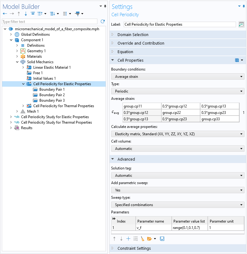
The Settings window for the Cell Periodicity feature.
The homogenized thermal conductivity can be established by applying the periodic boundary conditions on the temperature using the Periodic Condition feature in the Heat Transfer in Solids interface. The homogenized density and heat capacity can be computed based on the analytical mixing rules.
Step 4: Homogenized Material Properties
To compute homogenized density and heat capacity, the periodic boundary conditions are not needed. However, they are needed to compute the homogenized elasticity tensor, coefficient of thermal expansion, and thermal conductivity. The formulas for computing the homogenized properties are as follows:
Homogenized density (\rho_\textrm{h}):
where \rho_i is the density of ith constituent and V is the total volume.
Homogenized heat capacity (C_\textrm{h}):
where C_i is the heat capacity of ith constituent.
To compute the homogenized elasticity tensor, D_\textrm{h}, you need to run six different load cases where only one component of the average strain tensor is nonzero. The average traction vector at each load case is used to construct the homogenized elasticity tensor.
To compute the homogenized thermal expansion coefficient, \alpha_\textrm{h}, the RUC is subjected to the free expansion with unit rise in the temperature. \alpha_\textrm{h} is computed as:
where \mathbf{\epsilon}_\textrm{avg} is the average strain and T_\textrm{diff} is the temperature change.
To compute the homogenized thermal conductivity, k_\textrm{h}, you need to run three different load cases where the average temperature gradient is nonzero for each Cartesian direction. The average heat flux at each load case is used to construct the homogenized thermal conductivity.
The Homogenization App
Now let’s take a look at the Homogenized Material Properties of Periodic Microstructures app. The app’s user interface (UI) has six main elements: the ribbon and the Geometry, Materials, Information, Graphics, and Results windows. The video below show the app when it’s launched.
A video showcasing the UI of the app.
Below, we provide more information on these six elements within the app’s UI.
Ribbon
The ribbon has two different tabs, Home and Unit Cells. The Home tab includes the following buttons:
- Reset: resets the geometry, materials, or both
- Mesh: meshes the geometry with Normal, Fine, or Finer discretization
- Compute: computes the solution
- Export Material: exports the homogenized material into an XML-file or MPH-file. (This button doesn’t becomes active until the solution is available.)
- Reset Window Layout: resets the UI windows
- Report: autogenerates a report of the homogenization modeling. (This button doesn’t becomes active until the solution is available.)
- Help: links to the documentation
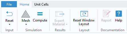
The Home tab in the ribbon. The Export Material and Report buttons are not yet available in this example.
The Unit Cells tab includes geometries for 10 different unit cells. You can click on the icon of any unit cell to use it.
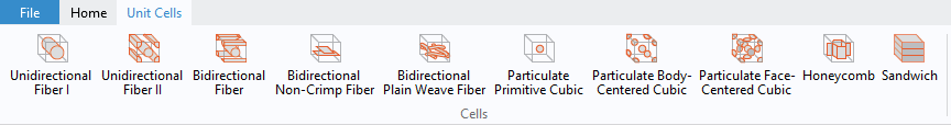
The Unit Cells tab in the ribbon.
Geometry Window
The Geometry window shows the changeable geometry parameters of the unit cell as well as a sketch of the geometry. It also includes the Build Geometry button.
Materials Window
The Materials window allows for selecting different materials for the constituents of the unit cell. It also includes options for selecting which homogenized properties to compute. There are ten different built-in materials from the Material Library in COMSOL Multiphysics® (see the list in the figure below). Additionally, there is a button for creating and editing user-defined materials. One thing to note is that the homogenized mechanical properties cannot be computed for air and water.
The app offers the following homogenized properties:
- Density
- Elasticity matrix
- Coefficient of thermal expansion
- Heat capacity
- Thermal conductivity
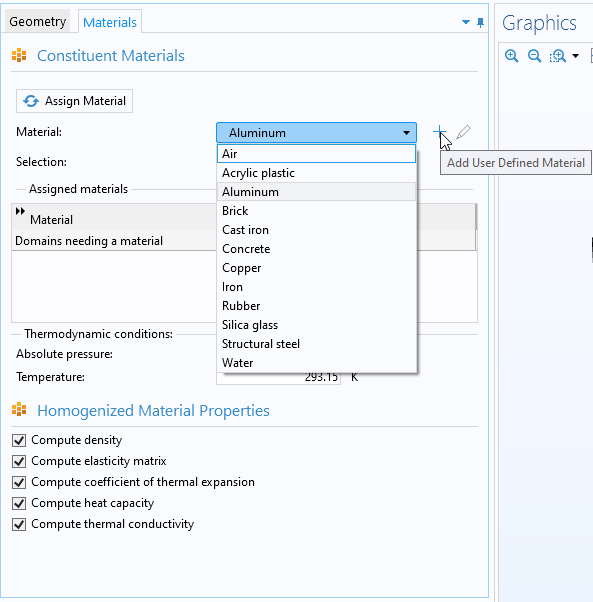
The Materials window in the app.
Information Window
The Information window shows the expected solution time and the expected memory usage. The window also shows the current status of the solution, geometry, mesh, and materials. Any changes in the app will be automatically updated here.
Graphics Window
The Graphics window in the app is consistent with the Graphics window in the COMSOL Multiphysics® UI. In addition to including the standard functionality, the window includes a button for hiding the matrix so that users can inspect the reinforcement constituent.
Results Window
The Results window shows the computed homogenized properties.
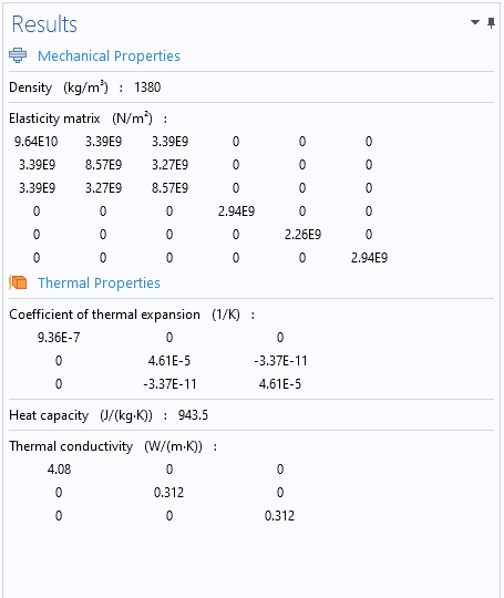
The Results window.
The Workflow
The step-by-step process for using the app can be summarized into the following steps:
- Choose an appropriate unit cell.
- Choose the appropriate geometric dimensions. Build the geometry.
- Assign correct materials to all constituents of the composite.
- Select different types of homogenized properties to be computed.
- Choose the appropriate mesh discretization.
- Check that the geometry, mesh, and materials have been updated in the Information window.
- Compute the solution.
Exporting and Importing Homogenized Material Properties
The main purpose of the app is to compute the homogenized properties of a composite that can be used in macromechanical analyses of composite structures. To do this, the computed homogenized properties from the app will need to be exported and then imported into a COMSOL Multiphysics simulation.
To export the results once the computation is finished, simply expand the Export Material menu in the ribbon and choose Export to MPH File or Export to XML File, depending on the file format desired. (The MPH output format can be imported into any COMSOL Multiphysics® version; the XML output format can be imported into COMSOL Multiphysics® version 3.5a onward.) In the file browser that pops up, choose the destination directory and a file name and then click Save.
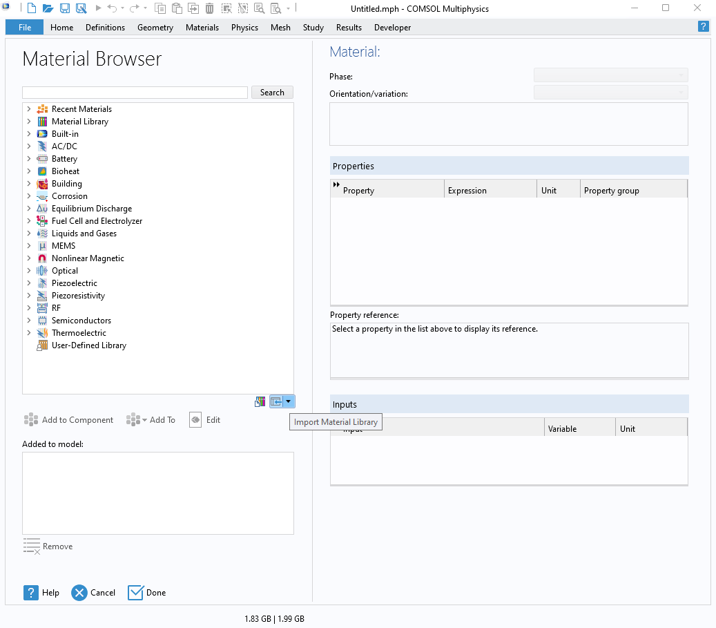
In COMSOL Multiphysics®, follow the steps below to import your custom material. You will need to have a model open to import the material. (This can be either a new or existing model.) In the ribbon, first select the Materials tab and then click Browse Materials.
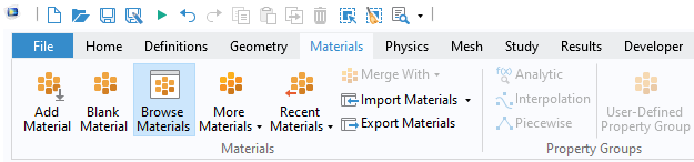
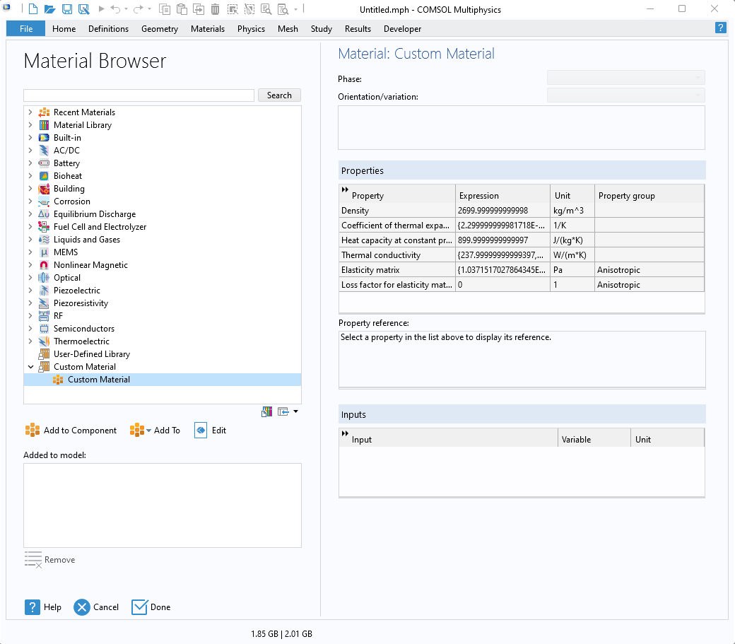
In the Material Browser window that opens, click the Import Material Library button. This launches a file browser where you can choose the previously saved MPH-file or XML-file. Thereafter, the custom material should appear in the list in the Material Browser.
Concluding Remarks
The simulation app discussed here computes homogenized material properties of various periodic microstructures and makes them available for import into COMSOL Multiphysics®. The app is advantageous for those who want to utilize the homogenized properties rather than focus on the underlying complexity of the modeling process.
For a technical guide covering homogenization in general, click the button below to be taken to the Learning Center.
Further Learning
- Try out the app yourself: Homogenized Material Properties of Periodic Microstructures
- For an in-depth guide to modeling composite materials, see this blog post: “Introduction to the Composite Materials Module”


Comments (2)
Said Bouta
April 28, 2024In the case of a composite material containing random fibers, can we apply the analytical models mentioned in the course page (https://www.comsol.com/support/learning-center/article/80311), where the fibers are either isotropic (and matrix) or anisotropic? Thank you for your explanations.
Amit Suresh Patil
April 29, 2024 COMSOL EmployeeDear Said,
There are different analytical models available in COMSOL, not all are applicable to all cases as there are different assumptions behind them. In the same course, we have shown one example where a numerical model of unidirectional composite is compared against the different analytical models, and there you can see how differently they behave. Coming back to your question, analytical model like Chamis, Halpin-Tsai, Halpin-Tsai-Nielsen are well suited to model randomly distributed isotropic or orthotropic fibers in an isotropic matrix.
Regards
Amit