Wave Optics Module Updates
For users of the Wave Optics Module, COMSOL Multiphysics® version 5.4 brings additional boundary conditions for the Electromagnetic Waves, Beam Envelopes interface for modeling thin dielectric layers, antireflective coatings, and mirror-like surfaces. Browse all of the Wave Optics Module updates in more detail below.
Transition Boundary Condition
A new Transition Boundary Condition feature for the Electromagnetic Waves, Beam Envelopes interface allows for the modeling of electrically thin layers and eliminates the need for a domain mesh. There are two options to choose from for the propagation direction. The first is Normal direction (default), which is useful for modeling thin metallic layers in mirror surface applications. The second is From wave vector, which is useful for thin dielectric layers, such as antireflective coatings. You can find this functionality used in the Beam Splitter model.
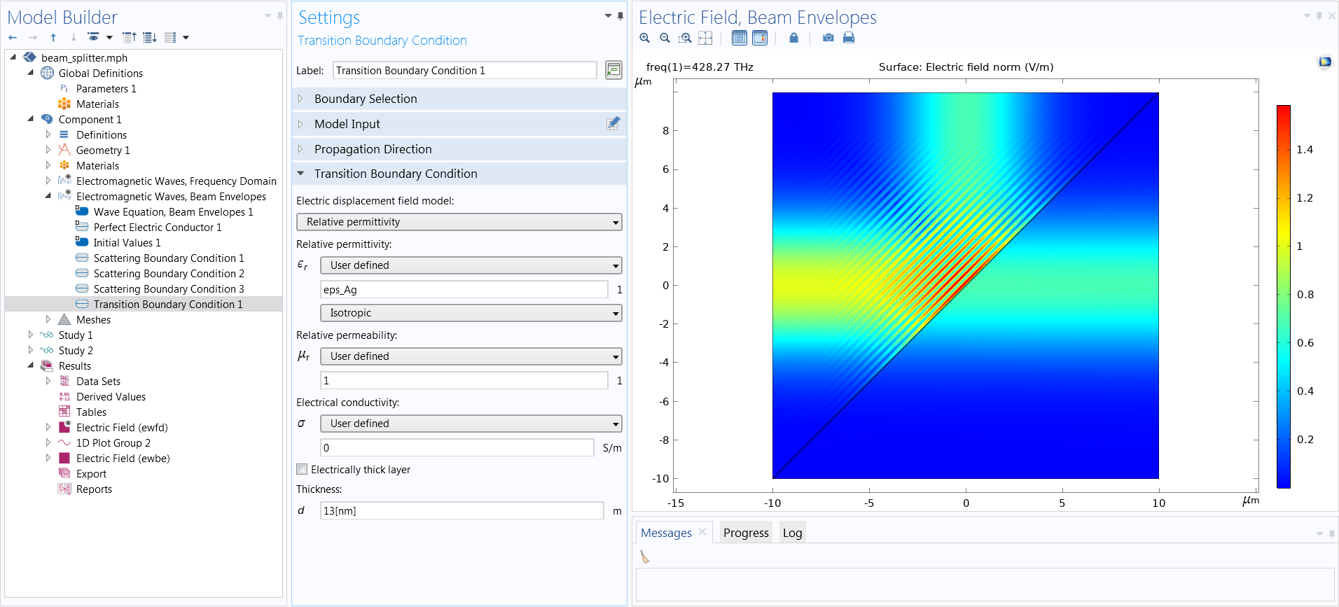
A Gaussian beam is incident from the left boundary, reflecting from, and transmitted through, a diagonal thin metallic layer, implemented using the new Transition Boundary Condition feature. The propagation direction is set to Normal direction.
Impedance Boundary Condition
A new Impedance Boundary Condition feature for the Electromagnetic Waves, Beam Envelopes interface allows for truncation of the simulation domain at an interface between two different material domains. There are two options to choose from for the propagation direction. The first is Normal direction (default), which is useful for exterior highly conductive materials such as metals. The second is From wave vector, which is useful for exterior dielectric layers such as glass substrates. You can find this functionality used in the Fresnel Equations model.
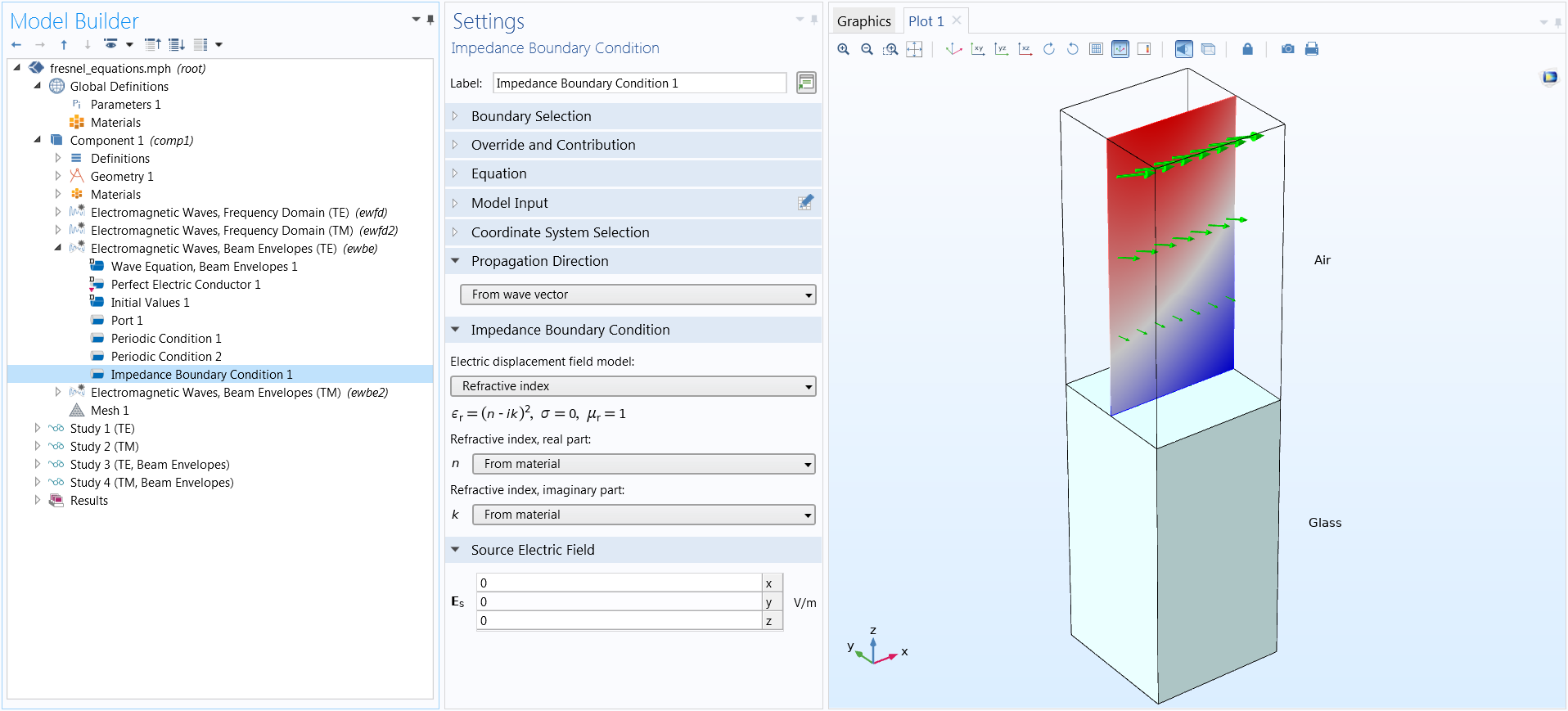
A plane wave is incident at an angle onto a glass substrate, reflecting at the boundary between the air and glass domains. The glass domain is replaced by the Impedance Boundary Condition feature. The propagation direction is set to From wave vector.
Slit Ports
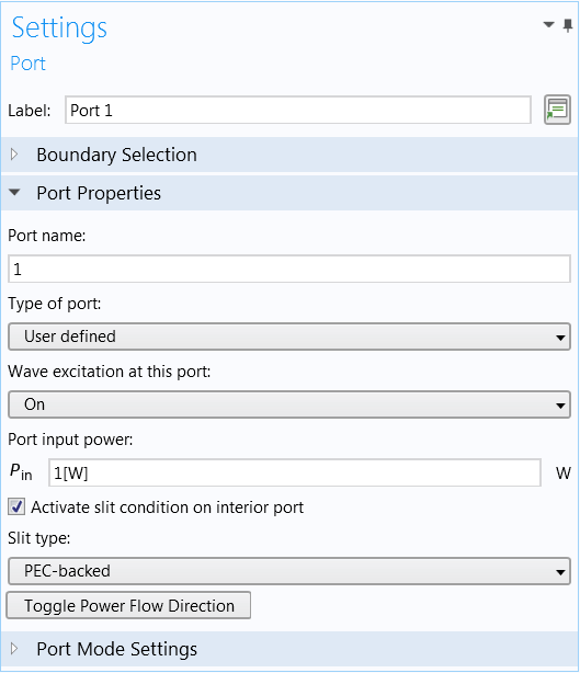
Slit Ports are now available for the Electromagnetic Waves, Beam Envelopes interface. A slit port is used on an interior boundary for exciting the computational domain with an incident wave and, at the same time, absorbing scattered waves matching the set port mode field. There are two important use cases. The first is when a perfectly matched layer (PML) backs the slit port, absorbing the remaining part of the scattered radiation that was not absorbed by the port; this is known as a PML domain-backed slit port. The second is when there is a regular port at one side and a Perfect Electric Conductor (PEC) boundary condition at the other side; this is known as a PEC-backed slit port.
PML-backed slit ports are useful when exciting a domain with a Gaussian beam, as the reflected Gaussian beam will not be perfectly absorbed by any port and instead a more general PML absorption method is needed. This is demonstrated and explained in the image and caption below. To implement this functionality, when the Port feature is applied to an interior boundary, you can click the Activate slit condition on interior port check box in the Settings window, as seen in the second image below.
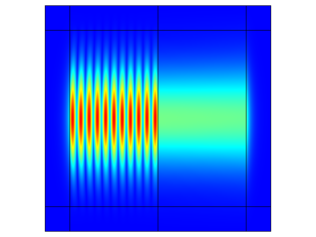 A PML domain-backed slit port is used on the left to excite a Gaussian beam. At the right, there is a listening PML domain-backed slit port. Most of the radiation is absorbed by the slit ports, with the remaining radiation absorbed by the PML.
One-Way Coupled Multiphysics in the Model Wizard
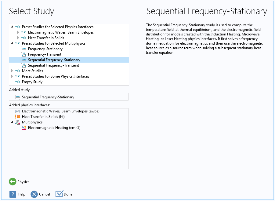
For multiphysics involving electromagnetic heating, such as Laser Heating in the Wave Optics Module or Microwave Heating in the RF Module, there are now two new study sequences available in the Model Wizard. The Sequential Frequency-Stationary study first solves a frequency-domain equation for electromagnetics and then uses the electromagnetic heat source as a source term when solving a subsequent stationary heat transfer equation. The Sequential Frequency-Transient study first solves a frequency-domain equation for electromagnetics and then uses the electromagnetic heat source as a source term when solving a subsequent time-dependent heat transfer equation. For both study sequences, it is assumed that the electromagnetics analysis does not depend on the computed temperature distribution. Whenever this simplifying assumption can be made, solving the two physics in a sequence requires fewer computational resources.
You can see this functionality used in the following models:
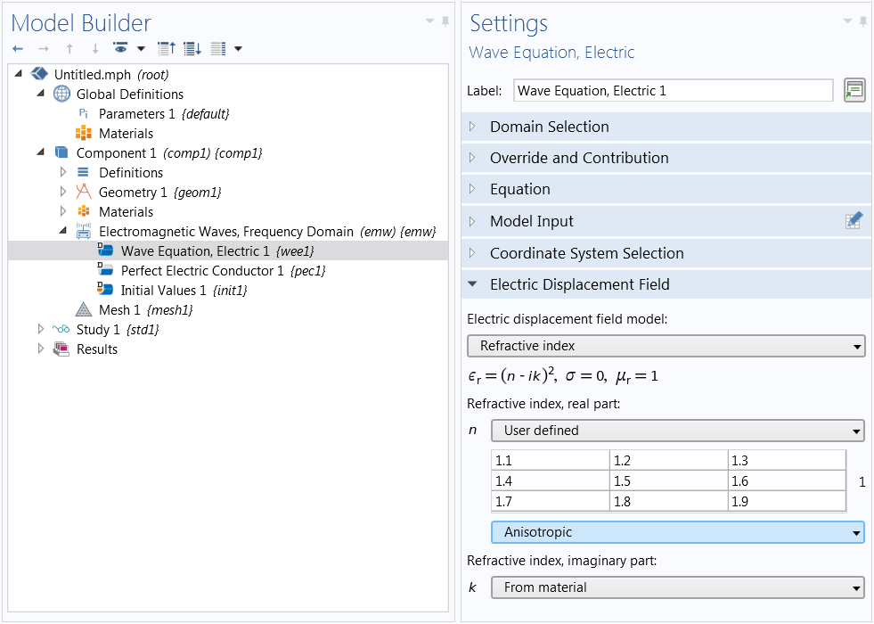
Fully Anisotropic Refractive Index
When the Refractive index option is selected for the Electric displacement field model combo box in wave equation features, you can now input a fully anisotropic tensor. A matrix-matrix multiplication is used to transform this refractive index tensor to the relative permittivity tensor.
More Interior Boundary Options in the Time Explicit Physics Interface
Perfect electric conductor (PEC), perfect magnetic conductor (PMC), and surface current density can now be applied to interior boundaries as well, when using the Electromagnetic Waves, Time Explicit interface.
Default Plots Changed to the RainbowLight Color Table
To improve legibility of the default black text appearing on parts of plots with lower numerical values, the default color table has been changed to RainbowLight.
The left plot uses the RainbowLight color table, whereas the right plot uses the previous default, Rainbow color table. It is clear that the black text is more legible on top of the RainbowLight plot.
Uniform Antenna Array Factor Function
It is now possible to evaluate the radiation pattern of an antenna array very quickly from the radiation pattern of a single antenna element by using an asymptotic approach that multiplies the far field of a single antenna with a uniform array factor. You can find this functionality in the updated Microstrip Patch Antenna model.
An 8x8 microstrip patch antenna array pattern synthesized from a single microstrip antenna simulation
3D Far-Field and RCS Functions from 2D Axisymmetric Models
By utilizing new far-field functions, a 2D axisymmetric model is now more useful for the purpose of quick estimation of the far-field response of the equivalent 3D model. A set of 3D far-field norm functions are available in a 2D axisymmetric geometry for the following cases:
- Antenna models using circular port excitation with a positive azimuthal mode number
- Scattered field analysis excited by the predefined circularly polarized plane wave type
Far-Field Norm Functions
| Description | Name | Full Name Examples | Full Name Description |
|---|---|---|---|
| 3D far-field norm | norm3dEfar | norm3DEfar_TE12 | Azimuthal mode number 1, TE mode circular port with mode number 2 |
| 3D far-field norm, dB | normdB3DEfar | normdB3DEfar_TM21 | Azimuthal mode number 2, TM mode circular port with mode number 1 |
More Far-Field Postprocessing Variables
New variables for computing the maximum directivity, gain, and realized gain have been added. These variables are available for global evaluation, without plotting a 3D far-field pattern. They can be accessed when the selection for the far-field calculation feature is spherical (in 3D) and circular (in 2D axisymmetry) and when the center is at the origin.
Far-Field Postprocessing Variables
| Description | Name | Available Content |
|---|---|---|
| Maximum directivity | maxD | 2D Axisymmetric, 3D |
| Maximum directivity, dB | maxDdB | 2D Axisymmetric, 3D |
| Maximum gain | maxGain | 2D Axisymmetric, 3D |
| Maximum gain, dB | maxGaindB | 2D Axisymmetric, 3D |
| Maximum realized gain | maxRGain | 2D Axisymmetric, 3D |
| Maximum realized gain, dB | maxRGaindB | 2D Axisymmetric, 3D |
Electrically Thick Layer in Transition Boundary Conditions
The new Electrically thick layer option decouples the two domains that are adjacent to a transition boundary condition. The boundary performs like an interior impedance boundary condition, but the layer geometry can be a surface rather than a domain.
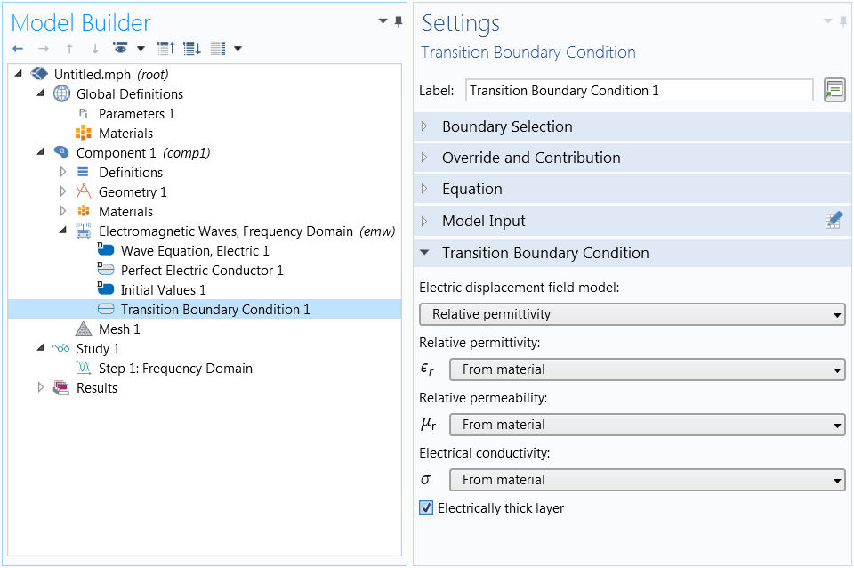
The check box for Electrically thick layer activates the decoupling between two adjacent domains.
Circularly Polarized Background Field for 2D Axisymmetry
A Circularly polarized plane wave option is now available for the scattered field formulation when modeling with a 2D axisymmetric component. To use this functionality, start by exciting an axisymmetric scatterer with a circularly polarized background field in a 2D axisymmetric model. Then, by using the norm3DEfar function, estimate the far field and radar cross section (RCS) of the same scatterer in 3D, illuminated by a linearly polarized background field.
 A 3D representation of a 2D axisymmetric model. The scattered field response of a 3D sphere, excited by a linearly polarized background field, can be estimated quickly by a 2D axisymmetric model with a circularly polarized background field.
Improved User Experience for Defining Ports
Arrow indicators now help to quickly identify which ports are inports (excitations) and which are outports (listeners). The arrow points in the direction of the power flow. An excited port is indicated by an inward arrow on the port boundary, while a listener port has an outward arrow. Lumped ports also support this visualization feature.
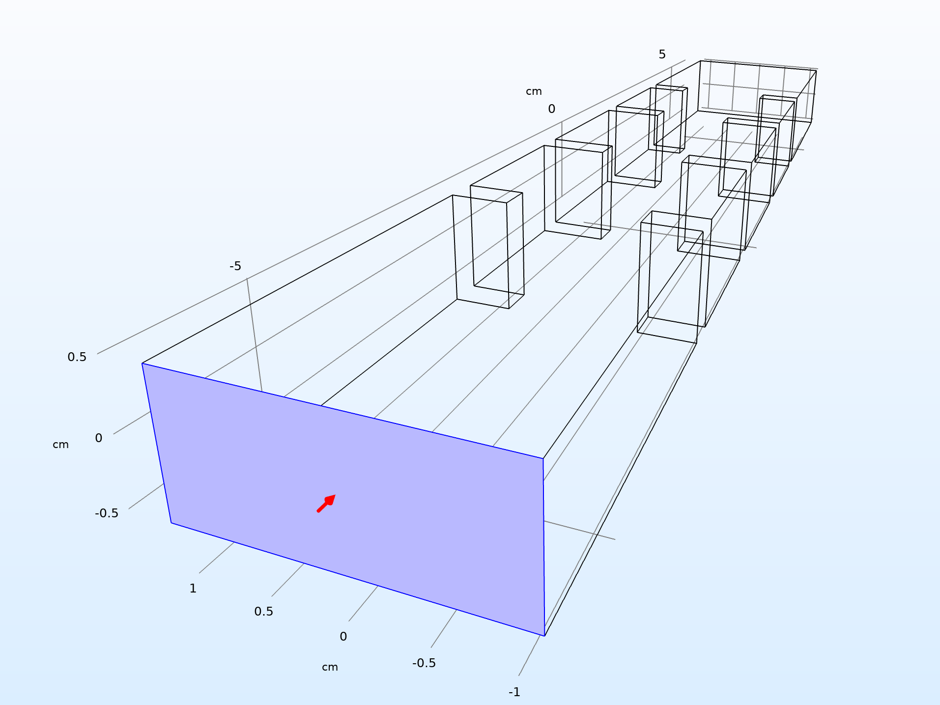 For the excited port boundary in this example model of an iris filter waveguide, the direction of power flow is shown as a red arrow.
New and Updated Tutorial Models
COMSOL Multiphysics® version 5.4 brings two new and one updated tutorial models.
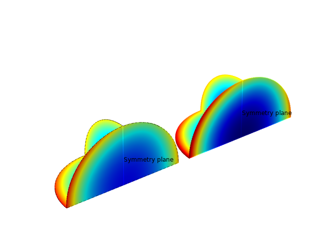
Optically Anisotropic Waveguide
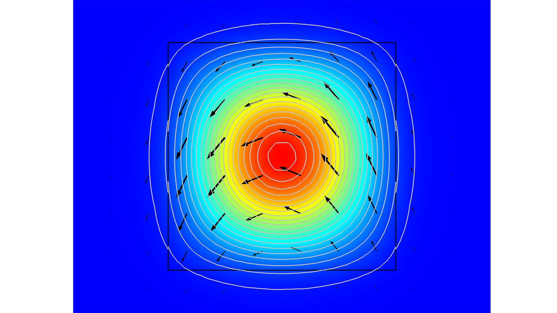 The lowest order mode in an anisotropic optical waveguide, where the optical axis points at a 45-degree angle from the direction of propagation.
Search in the Application Library:
optically_anisotropic_waveguide
Focusing Lens
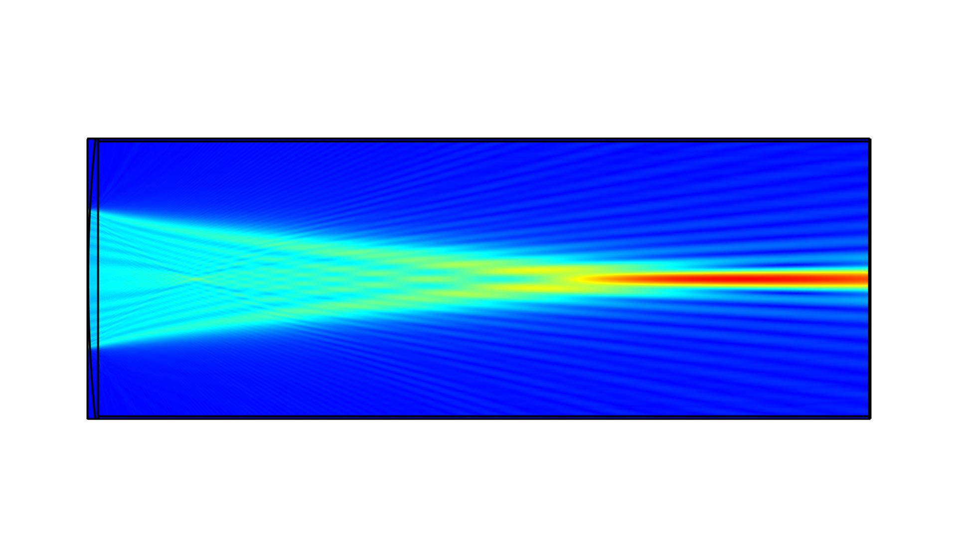 A plane wave is focused by a lens (in the left part of the domain) to a focal point in the right part of the domain.
Search in the Application Library:
lens_waveguide
Directional Coupler with Two Copropagating Modes
 This updated model demonstrates the ability to solve for the amplitudes of two modes that have different propagation constants, but in the same direction, allowing for a very coarse mesh in the direction of propagation.
Search in the Application Library:
directional_coupler