Studies and Solvers Updates
COMSOL Multiphysics® version 5.5 includes cluster computing improvements, new mesh adaptation functionality, faster solvers, and more. Learn about all of the updates relating to studies and solvers below.
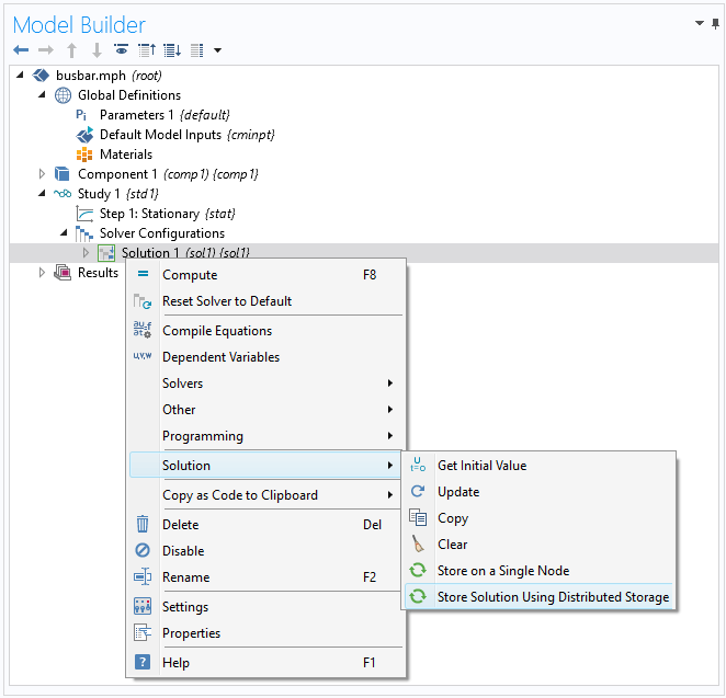
Distributed Solution Data Storage on Clusters
For improved efficiency when saving solutions on a cluster, you can now right-click a Solution node and choose Store Solution Using Distributed Storage. This will store the solution using a distributed Input/Output method, which can improve performance by reducing disk requirements when storing many solutions (many time steps or frequencies).
Multigrid Performance
The setup of the smoothing operations for the multigrid solvers are improved on clusters. This leads to improved performance for virtually all multigrid-dependent simulations that solve linear systems over and over again. The improvements also have effects, albeit smaller, when running on one node (not cluster). For comparison, for a particular type of hardware, the Ahmed body model is 15% faster on a single node (50 minutes vs. 60 minutes) and 30% faster on 6 nodes (40 minutes vs. 60 minutes) compared to COMSOL Multiphysics® version 5.4.

Algebraic Multigrid Improvements
A new Lower element order first (any) setting is available for the algebraic multigrid (AMG) and smoothed aggregation AMG (SAAMG) solvers. It makes it possible to use a combination of solvers: first the geometric multigrid (GMG) solver with lower order until order 1 is reached and then the AMG or SAAMG solver to generate the coarser levels in a multigrid approach. The advantage with the new setting is that you can control the total number of multigrid levels in one setting and that you do not have to repeat the pre- and postsmoother settings in two places.
Discontinuous Galerkin Method
Improvements to the method used for storing the solution object makes the discontinuous Galerkin method more efficient. Less data needs to be communicated, which makes the method faster and more memory efficient on clusters. For comparison, a large acoustics benchmark model is 30% faster (700 seconds vs. 980 seconds) compared to version 5.4 when running on 6 nodes. This improvement applies to the Wave Form PDE interface and the physics interfaces, available in add-on modules, based on the discontinuous Galerkin method.
New Schur Solver for Domain Decomposition
A new Domain Decomposition (Schur) solver is now available to provide domain decomposition using an exact Schur complement and an algebraic hybrid direct-iterative solver. This method is useful, for example, when solving strongly coupled multiphysics problems where a direct solver would be preferred but cannot be used due to memory consumption. The Domain Decomposition solver available from earlier versions of COMSOL Multiphysics® is now available as Domain Decomposition (Schwarz).
The Schur solver solves a linear system of equations with a strategy that resembles that of a direct solver by using local Schur matrices and their inverses. A distributed version of the solver is used on clusters. The system matrices used by the Schur solver are in the solver stage used to solve the global Schur matrix problem iteratively. After this stage, the local problems can be solved independently using any solver, but they should typically be solved by a direct solver like MUMPS. The Domain Decomposition (Schur) solver is relatively expensive compared to an optimal iterative solver, but can be more efficient than a direct solver on clusters.
Plot Undefined Values for Assembled Residual and Jacobian Matrices
You can now plot the coordinate locations of undefined values introduced during the assembly of a residual vector or a Jacobian matrix. This can be used to more easily understand the source of such undefined values during the modeling process.
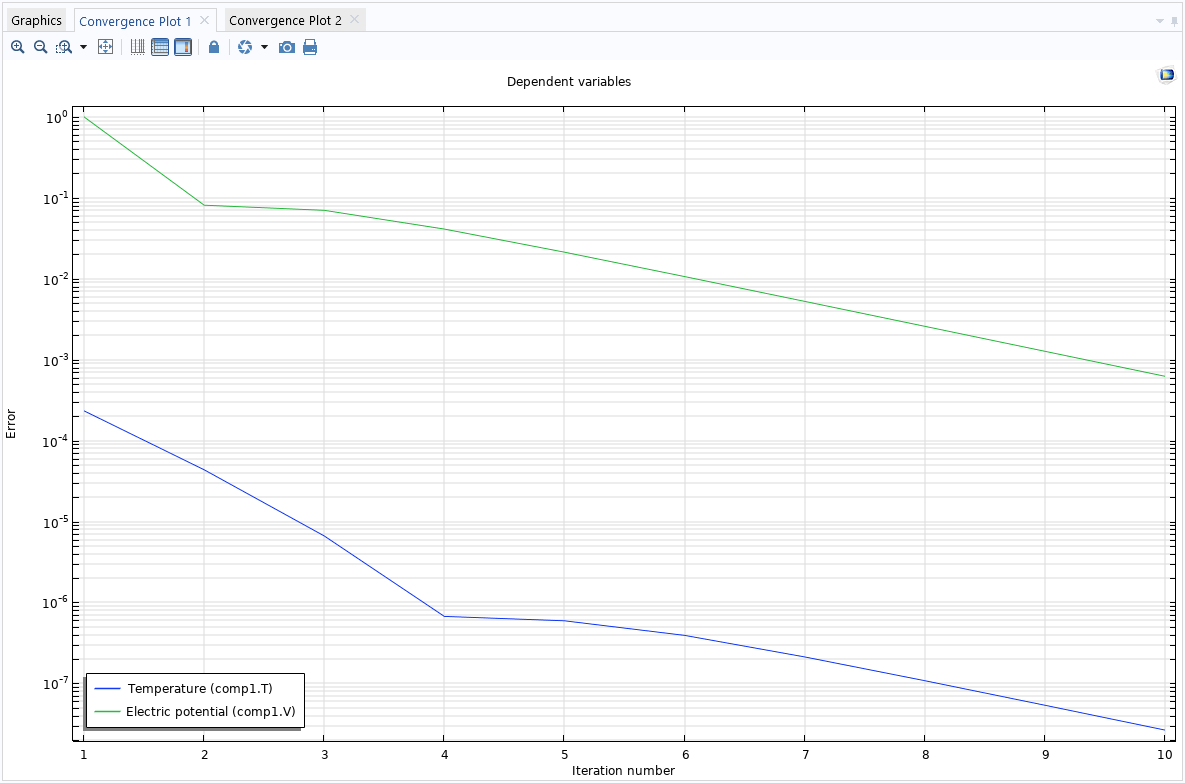
Error Estimates in the Convergence Plot for Nonlinear Solvers
You can now get a log and plot of error estimates per field and state during the solution for applicable multiphysics models if you select Detailed from the Solver log list in the Advanced node’s Settings window. This functionality is available for the Fully Coupled and Segregated solvers.
Mesh Adaptation Improvements
For adaptive mesh refinement, it is now possible to choose on which geometric level the mesh adaptation will be performed, so that you can do adaptive mesh refinement on surfaces, for example. You specify the geometric entity level in a new Geometric Entity Selection for Adaptation section in the main study step's Settings window. In that section, you can also select for which domains or surfaces, for example, to perform the mesh adaptation (that is, you can do adaptive mesh refinement in a subset of the geometry).
It is now possible to add a number of global goal-oriented quantities to make the mesh adaptation terminate when those quantities are stable to a requested accuracy. These goal-oriented quantities could, for example, be the S-parameters for an RF simulation. The goal-oriented termination can be used for any error estimation method supported by the adaptation and error estimates algorithm. Choose Manual from the Goal-oriented termination list under Adaptation and Error Estimates in the study step's Settings window to enter user-defined goal-oriented quantities and their tolerances.
For time-dependent adaptive mesh refinement, the General modification method and Rebuild mesh methods are now available in the Adaptive Mesh Refinement node's Settings window. The general modification method can resolve sharp fronts with fewer mesh elements in total compared to the previous methods.
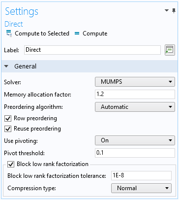
Block Low-Rank Factorization
The MUMPS solver has been upgraded and now supports blocked low-rank factorization, both when computing the LU factors and when storing them. This is an approximate, but accurate LU-factorization method that can reduce memory consumption when solving. You activate it by selecting the Block low rank factorization check box in the Settings window for the MUMPS direct solver. The solution time and memory usage for certain structural mechanics and acoustics models can be reduced by as much as 25% compared to the default standard factorization.
New Scaling Type for Eigenmodes
You can now specify a maximum value for the scaling of eigenvectors in the Settings window for the Eigenvalue Solver node by choosing Maximum from the Scaling of eigenvectors list and then entering a value in the Maximum absolute value field. The peak value is then normalized to that value. You can use this setting to keep eigenmodes small.
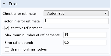
Termination of Iterative Improvements for the Direct Solvers
For the direct solvers (PARDISO, MUMPS, and SPOOLES), it is now possible to stop iterative improvements if the residual is not reduced by using the new Error ratio bound setting in the Error section of the solver's Settings window. By default, it is set to 0.5 (valid values are between 0 and 1; a lower value means that the iterations terminate more quickly). When the Check error estimate setting is set to Automatic, a single warning that reads "Iterative refinement triggered" appears in the Log window if the iterative refinement is triggered.
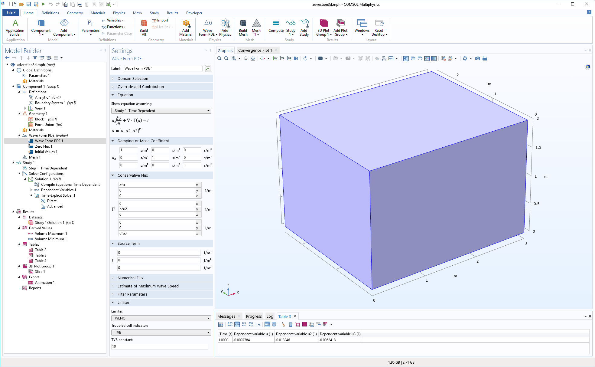
Limiters for the Discontinuous Galerkin Method
When computing discontinuous solutions to conservation laws, for example, when using the Wave Form PDE interface, spurious oscillations and instabilities might arise. For controlling oscillations around discontinuities and stabilizing the computations of (nonlinear) conservation laws, a weighted essentially nonoscillatory (WENO) limiter is now available for the discontinuous Galerkin method available in the Wave Form PDE interface, as well as the time explicit interfaces in the Acoustics Module, RF Module, Wave Optics Module, Structural Mechanics Module, and MEMS Module.
New Batch Options
There are two new command-line options when running in batch mode from the operating system command line. The option -batchlogout is used to also direct the log to standard out when the log is stored on file using the option -batchlog . The option -norun is used for not running the model and can be used, for example, to clear the solution or mesh, using the option -clearsolution or -clearmesh, respectively, without having to wait for the model to solve.